Evolutionary Shape Optimisation

Evolutionary Shape Optimisation

Using a Voxel Based Representation.

Peter James Baron

MSc Information Technology: Knowledge Based Systems

Department of Artificial Intelligence

University of Edinburgh

1997

Abstract

Shape optimisation within constraint limits is a hard problem from the field of Mechanical Engineering. The objective is to design a shape which best satisfies some predetermined goal whilst at the same time observing some constraints. Much work has been done on various problems within this domain [Bentley 96][Chapman et al. 94] [Smith 95a][Watabe & Okino 93], however the majority to-date has focused on parametric and other highly restricted representations of the shapes being optimised. This thesis describes experiments performed using a voxel based representation and an evolutionary optimisation algorithm. As any attempt to perform shape optimisation using an unrestricted object representation must use a highly effective evaluation function in order to be able to deal with the varieties of design that an evolutionary optimisation algorithm may produce, the work detailed here was intended to first design and test suitable operators to deal with the extremely large chromosomes required by a voxel representation, and by then extending the work to permit evaluation from a commercial Finite Element analysis package, it was expected that the program would be able to perform real-world shape optimisation tasks with very few restrictions on the shapes being tested. The results obtained indicate that it is possible to circumvent the difficulties presented by a voxel representation [Watabe & Okino 93], and that with suitable operators, useful and unexpected results can be gained from a real-world optimisation task.

Acknowledgements

I would like to thank my primary supervisor Dr. R. Fisher for his guidance, advice and assistance throughout all of the stages of this project. I would also like to thank Dr. F. Mills of the Department of Mechanical Engineering for his assistance with the Mechanical Engineering side of things, and Andy Sherlock at the Department of Mechanical Engineering for his invaluable advice and his willingness to help with any and all aspects of the project.

During the past three years Andrew Tucson has been an invaluable source of useful knowledge, good advice and friendship, and for these gifts I wish to express my sincere appreciation.

Finally I want to thank Julie Humphrey who has constantly reassured me that the effort is worthwhile and without whom it might not have been.

Contents

1 Introduction 1

1.1 Introduction to the problem . . . . . . . . . . . . . . . . 1

1.2 Approach taken . . . . . . . . . . . . . . . . . . . . 2

1.3 Contributions made by this work . . . . . . . . . . . . . . 5

1.4 Outline of this thesis . . . . . . . . . . . . . . . . . . 5

2 Background and previous work 8

2.1 The problems to be addressed . . . . . . . . . . . . . . . 8

2.2 The genetic algorithm . . . . . . . . . . . . . . . . . 11

2.2.1 Other search techniques . . . . . . . . . . . . . . . 12

2.2.2 Advantages of the genetic algorithm . . . . . . . . . . . 15

2.2.3 The standard genetic algorithm . . . . . . . . . . . . . 16

2.3 Introduction to shape optimisation . . . . . . . . . . . . . 19

2.3.1 The stress analysis model mathematics . . . . . . . . . . 20

2.3.2 Possible approaches to shape optimisation . . . . . . . . . 21

2.3.3 The voxel based approach to shape optimisation . . . . . . . 22

2.4 Miscellaneous relevant work on GA based shape optimisation . . . 24

2.5 Conclusions . . . . . . . . . . . . . . . . . . . . 25

3 Design and testing of new operators 27

3.1 The one-dimensional experiments . . . . . . . . . . . . . 27

3.2 A two-dimensional representation of a beam cross-section . . . . . 31

3.3 The GA experiments . . . . . . . . . . . . . . . . . 32

3.3.1 Experiments using the naïve GA . . . . . . . . . . . . 33

3.3.2 Results obtained from the naïve GA . . . . . . . . . . . 33

3.3.3 Experiments with the rank selection pressure . . . . . . . . 36

3.3.4 Experiments with the constraint penalty multiplier . . . . . . 40

3.3.5 Experiments with a dynamically changing constraint penalty

multiplier . . . . . . . . . . . . . . . . . 46

3.3.6 A new operator: smoothing . . . . . . . . . . . . . . 53

3.3.7 An n-dimensional crossover operator . . . . . . . . . . . 56

3.3.8 An n-dimensional mutation operator . . . . . . . . . . . 60

3.3.9 Dynamic mutation operator probabilities . . . . . . . . . . 63

3.3.10 Comparison of modified GA with naïve GA . . . . . . . . 66

3.4 Conclusions about the simplified physics model experiments . . . . 68

4 Transferring the solutions to real problems 71

4.1 Motivation for this approach . . . . . . . . . . . . . . . 71

4.2 The annulus design problem . . . . . . . . . . . . . . . 72

4.3 Implementation details . . . . . . . . . . . . . . . . . 73

4.4 Results from the basic system . . . . . . . . . . . . . . 77

4.5 Improvements made to the system . . . . . . . . . . . . . 82

4.6 Conclusions about the real-world system . . . . . . . . . . . 90

5 Conclusion 92

5.1 Summary of conclusions . . . . . . . . . . . . . . . . 92

5.2 Further work . . . . . . . . . . . . . . . . . . . . 94

Appendices 95

A Rolls Royce annulus problem specification 95

B Ansys macro listings 99

B.1 Full optimisation macro mask listing . . . . . . . . . . . . 99

B.2 Single optimisation macro listing . . . . . . . . . . . . . 109

C Results log files 110

C.1 Log of basic GA results on annulus problem . . . . . . . . . . 110

C.2 Log of improved GA results on annulus problem . . . . . . . . 116

Bibliography 123

Chapter One.

Evolutionary Shape Optimisation Using a Voxel Based Representation.

1.1 Introduction to the problem.

Shape optimisation is the process of attempting to discover the optimum shape to perform some given task, frequently within some pre-determined constraints. In some simple cases the solution may be readily apparent, even trivial, for example; to maximise volume and minimise surface area the shape required is a sphere. However in most cases the solution is not so easily found. Engineering knowledge and a sound understanding of the underlying physics of a problem may enable a well-trained person to make a good guess as to a suitable form, but this leaves open the possibility of major improvements being totally overlooked and may not be sufficient if the problem being addressed is very highly constrained.

This thesis examines two different shape optimisation problems and will attempt to show that the combination of genetic algorithms with suitable operators and a voxel based representation, forms an effective tool for solving this type of problem.

The first optimisation addressed in this thesis is that of minimising the amount of mass in load-bearing beams, whilst ensuring that the maximum stress they are capable of withstanding remains above a given minimum level. This is tackled first by means of a mathematical model which contains some simplifying assumptions about the physics of the situation. Although this is not very realistic in terms of a real-world analysis, it has the advantage of being very quick to run which makes it a suitable test-bed for experimentation with the operators and the parameters of the GA being used.

The second optimisation is that of designing a minimum mass annulus for a jet-turbine engine which must withstand several different forces without exceeding the maximum stress limits in any one of several key areas. This problem does not have any simplifying assumptions, and so is analysed in full by a commercial Finite Element analysis package; Ansys 5.3* . As the evaluation function is very time-consuming it was necessary to design several new GA operators which increase the rate of improvement considerably.

Previous work in this field includes:

n [Bentley 96] which has successfully evolved a wide range of shapes and structures using geometric primitives as building blocks.

n [Chapman et al. 94] which addresses issues in structural topology design using pixels as design primitives with a standard GA.

n [R Smith 95a] which uses a GA with a parametric representation to optimise the same annulus problem covered in Chapter 4 of this thesis.

A more detailed description of shape optimisation and stress analysis will be presented in Chapter Two.

1.2 Approach taken.

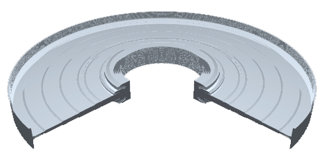
The representation of the problem space chosen for this work is that of voxels+ , which are a method of partitioning the search area or volume into rectangular regions or boxes which are then assigned a binary full/empty value.

A Voxel Representation of a Part. The Original Part.

Figure 1.1

This approach has many advantages over the alternatives including:

n The ability to represent any shape without restriction.

n The ease with which an existing engineering solution can be converted into voxels.

n A natural mapping to the traditional binary chromosomal representation frequently used by GAs.

n The simplicity with which domain knowledge can be integrated into the solution.

However in [Watabe & Okino 93] the authors object that voxels suffer from several apparently fatal weaknesses when used to represent this type of problem including:

n The occurrence of small holes in the final shape.

n The long length of the chromosomes.

n The expectation that cross-over would be ineffective.

n The lack of smoothness in the final shape’s outline.

It will be shown during the early experiments described in Chapter 3 that these objections do not constitute a problem when addressed with appropriate operators and GA optimisations.

The choice of voxels as a representational form was motivated by several key points. The previous work which has made use of voxels has tended to either avoid using domain knowledge in the operator design, or has concentrated on very low resolution voxel grids in an attempt to avoid huge chromosomes. Voxels also offer some important advantages over other representations, including the ability to generate unexpected designs, the ease with which the user can initialise the population to the previous best solution and quick incorporation of domain knowledge in the form of areas of voxels with fixed values.

Genetic Algorithms (GAs) have proven themselves to be a highly flexible search technique, able to find good solutions to a diverse range of problems in many different fields [Goldberg 89]. They use evolutionary computation techniques to search large and difficult fitness landscapes in order to find near-optimal solution vectors.

[Michalewicz 92] describes “evolution programs” as a sub-class of the range of algorithms which rely on analogies to natural processes. In [Michalewicz 92] he writes:

“… a population of individuals (potential solutions) … undergoes a sequence of unary … and higher order … transformations. These individuals strive for survival: a selection scheme biased towards fitter individuals selects the next generation. After some number of generations, the program converges - the best individual hopefully represents the optimum solution.”.

In this thesis the term GA will be substituted for Michalewicz’s “evolution programs” to reflect the fact, widely recognised in the field of evolutionary computation, that the original definition of GA (as using only binary chromosomes, simple crossover and bitwise mutation) is far too narrow and explicit to encompass this rapidly growing field.

As the nature of the voxel representation leads inevitably to extremely large search areas the use of GAs is an obvious choice. A further introduction to the theory of GAs can be found along with a more detailed description of shape optimisation, stress analysis and the voxel based representation in Chapter 2.
1.3 Contributions made by this work.

During the first set of experiments a number of new and modified operators were designed and tested, and some of them proved to be extremely effective at reducing the amount of time taken for the GA to achieve a good solution. Several other operators were found which directly address the issues raised by [Watabe & Okino 93] and solve the problems described by them.

The second set of experiments extends the range of previous work in this domain to use a commercial FE package to perform the optimisation. Two sets of experiments were performed, firstly a simple adaptation of the GA to the new problem was tested. Although these experiments did discover some difficulties when using Finite Element Analysis with a voxel based representation, further work resulted in the design of a set of solutions to those difficulties and some very interesting results were obtained from the analysis.

The work in this thesis will show that a genetic algorithm using a voxel based representation, whilst suffering from several difficulties, is by no means an implausible approach to the problem of shape optimisation. The benefits obtained by using this representation may in many cases out-weigh the disadvantages, thus making it an appropriate technique for optimisations where the optimum is unknown or where engineering insights are to be used to assist the process.

1.4 Outline of this Thesis.

The task was addressed as a series of experiments, each of which built on the results of the previous steps; the format of this thesis reflects this approach, with the majority of the work being presented in the order of experimentation and with appropriate comments where one set of experiments suggested the approach to be taken next.

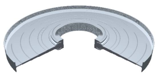
Final Annulus Design from the Results Set.

Figure 1.2

The majority of Chapter 2 deals with the background explanations of GAs, shape optimisation and stress analysis necessary to understand the rest of the thesis. An investigation was then made into the current state of the art in shape optimisation, with particular reference to the use of GAs to perform the search. The results of this study are presented in Section 2.3.

Initially, a two dimensional shape optimisation problem was undertaken using simplifying assumptions in the stress analysis model. This allowed rapid evaluations of the shapes produced by the GA, thus permitting in-depth investigation into the effectiveness of various modifications to the basic optimisation technique. A description of these experiments, their results, and the optimisations made can be found in Chapter 3.

Once the GA code was running effectively on this simplified problem, the level of realism in the stress analysis model was increased by using a commercial Finite Element package to perform the shape evaluation. At this point the experiments were using a realistic representation of all stresses involved in the shapes generated by the GA. Chapter 4 gives details of the approach taken, the results and the difficulties encountered during this final stage of the experimentation.

Chapter 5 contains the conclusions arrived at during this study and the recommendations for future work.

The Appendices include details of the annulus design problem specification, the macros uses to make Ansys perform the optimisation and some results data files.

Chapter Two.

Background and Previous Work:

2.1 The problems to be addressed.

The first optimisation addressed in this thesis is the design of a beam cross-section which minimises the amount of material in the beam, whilst leaving it capable of supporting a given minimum mass. This problem will be approached using a simplified model of the physics involved in order that the speed of evaluation is as fast as possible. The second optimisation is the design of an annulus for the centre of a jet-engine’s turbine propeller, which must be as light as possible but still be able to withstand stresses in two different directions at various key positions. This will be evaluated using a full commercial Finite Element Analysis (FEA) package in order that all of the forces and stresses experienced by the part are simulated as accurately as possible.

The beam optimisation was chosen as an example of a sufficiently hard problem that, even when using a simplified model of the physics involved, the solution surface would be extremely complex. An additional reason for the choice of this problem is that a good solution is well-known to engineers. The ‘I’ beam (shown in Figure 2.1), which is commonly used in sky-scraper construction, is generally accepted as being a good form for a beam cross-section to gain maximum strength for minimal mass.

Issues to be addressed in this optimisation were;

n How well does a standard GA perform on a complicated problem using a voxel representation?

n Can operators be designed that overcome any perceived flaws in the standard GA?

n What alternative operators can be designed to improve the GA performance in regards to voxel based optimisations?

n What adjustments should be made to the balance of operators to further increase the rate of optimisation?

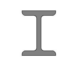
An ‘I’ Beam Cross-Section.

Figure 2.1

The annulus design problem is specified in detail in a document supplied by Rolls Royce to Richard Smith during his time with the Mechanical Engineering department of Edinburgh University, which is included as Appendix A. As specified by Rolls Royce, the annulus design is very tightly constrained, ie: the figures given for maximum stress represent a reasonably good solution. This was expected to cause some difficulties as a random population initialisation would probably create an initial population which contains only invalid solutions.

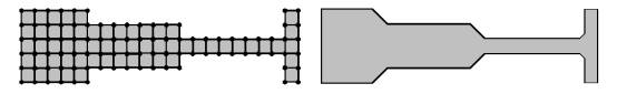
The choice of a voxel based representation was expected to raise some difficulties when the solutions produced were analysed by the FE package. This is because FEA does not cope well with sharp corners and will normally not use uniformly sized meshes. Voxels are by definition uniform in size, and though it would in theory be possible to subdivide edge voxels into a finer grid, the FE package used for this analysis (Ansys v5.3) could only recognise elements which connect at their major vertices. Thus in order to subdivide the voxels into a finer grained mesh would involve at least one intermediate step and a lot of extra processing, as seen in Figure 2.2.

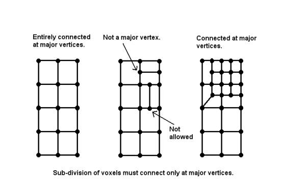
Figure 2.2

One further issue was of concern at the beginning of the experimental work described here; what would be the best way of getting Ansys 5.3, a commercial, stand-alone, GUI driven FE package, to perform the analysis of the GA produced voxel shape representations? This was a particularly worrying problem as all of the work was performed on PC compatible machines, which are not noted for the flexibility of their inter-process communications systems.

These problems and their solutions are described in detail in Chapter Three for the beam and Chapter Four for the annulus optimisation.

2.2 The genetic algorithm.

`Genetic Algorithm’ is the term which has come to cover the use of evolutionary directed algorithms for searching complex parameter spaces to find a near-optimal solution. This technique requires the formulation of a suitable `fitness’ function which can evaluate any solution possible within the representation chosen and return a valid fitness score. The search is performed by maintaining a population of potential solutions and allowing them to interbreed (crossover), mutate and die. The selection of survivors from one generation to the next is based on each individual’s fitness score relative to the population as a whole, thus those individuals with better fitness scores have a higher probability of surviving and breeding in the next generation.

The sequence of data which represents an individual member of the population of solutions is called a chromosome, taking its name from the DNA sequence in humans as this whole technique is based on an analogy to nature’s evolutionary processes. Each item of data in the chromosome is called a gene following the same naming convention. Genes in a traditional GA are single bits, however floating point numbers and more complicated data types have also been used [Michalewicz 92] (pages 2-9) and [Davis 91].

Crossover is the process of taking some genes from one `parent’ and swapping them with the genes in the same position on the chromosome of the other parent. This has the effect of propagating short gene sequences throughout the population and as the chromosomes are more likely to reproduce if they are fit, only sequences which make chromosomes fitter will spread through the population. Mutation is the method whereby new genetic variations can enter the population and generally consists of randomly changing the value of a small number of randomly chosen genes.

A more complete description of the theory and implementation details of conventional genetic algorithms can be found in [Holland 75], and [Michalewicz 92] (Chapter Five) includes details of some of the possible modifications to the basic approach which extend the power and capabilities of this optimisation technique.

2.2.1 Other search techniques.

Exhaustive search is the procedure of iteratively supplying an evaluation function with every single parameter setting within the scope of the problem being studied. It is impossible to do this in a reasonable amount of time for most real-world problems due to the range and the number of parameters which define the problem. In a voxel based representation of a beam using a two-dimensional grid divided into 32x64 voxels, the total problem space is 2 ²⁰⁴⁸!

Random search involves iteratively trying different randomly selected parameter settings whilst always remembering the best solution found. For large problem spaces this is ineffective due to the small probability of randomly choosing good parameter settings, this is especially true when a large portion of the solution space constitutes invalid solutions due to violations of the problem constraints.

Stochastic hill-climbing (SHC) is an optimisation technique based on the concept of hill-climbing. In a well-behaved function optimisation problem, the solution space may often be visualised as a smooth surface in multiple dimensions as shown in Figure 2.3. Given a randomly selected initial parameter setting, a steepest-ascent hill-climbing algorithm will evaluate the solution function and find a single point on the surface. By varying the problem parameter settings and re-evaluating the function, other points can be found which will either be worse, the same or better than the previous solution. Repeatedly varying the parameters and keeping the best solution from a set as the starting point for the next iteration will result in continual progress up the hillside, when no solution is better than the current starting point the algorithm has achieved an optimal solution.

The type of problem which can be solved by hill-climbing in this simplistic formulation is highly limited. Most real-world problems involve far more complex solution surfaces with many bumps and pits which represent local optima as seen in Figure 2.4.

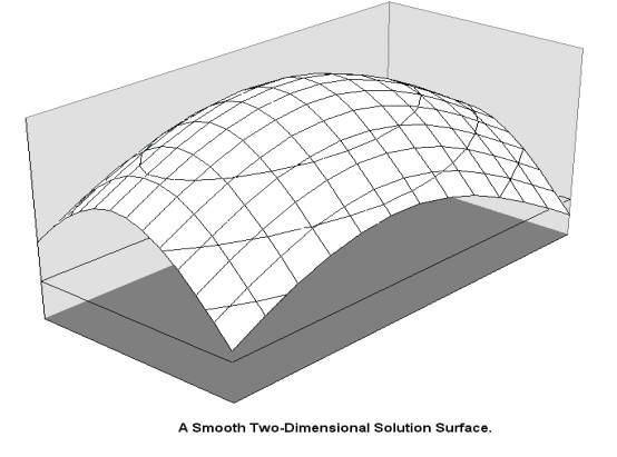
Figure 2.3

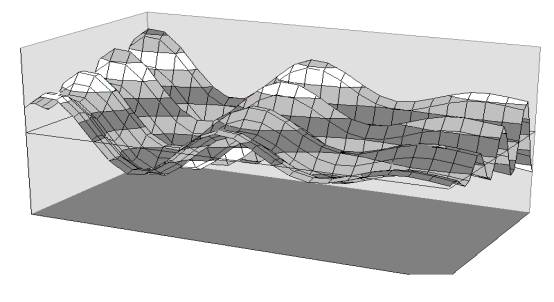
Uneven Solution Surfaces May Have Many Local Optima.

Figure 2.4

SHC attempts to address these more complicated problems by adding the capability to randomly reinitialise the current starting point when no more improvement is possible from the position found. The best solution found is continually recorded, so that after a given number of iterations the SHC can report the parameter settings which produced that solution.

A major problem with SHC is that when a solution space with a very large number of local optima is faced, the chance of a random re-initialisation of the parameters producing a solution which is on the same hill as the global optima is very small. Another problem is encountered when constraints are applied to the solution space. Figure 2.5 shows a very simple optimisation problem which has been complicated by the addition of a constraint limitation. SHC can only find the optimum for this problem if it starts somewhere on the line going straight up the hill through it. From this it is apparent that the probability of SHC finding a good solution is reduced drastically by the addition of problem constraints.

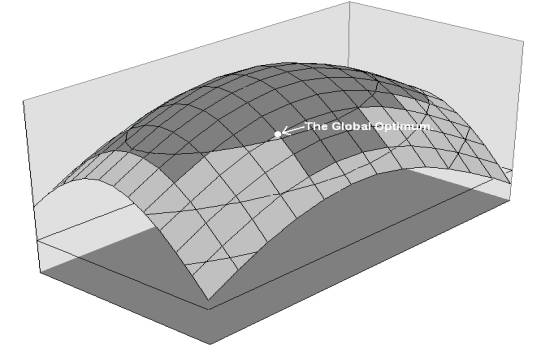
Constraint Limitations Cause Difficulties For Hill Climbers.

Figure 2.5

Simulated annealing is an approach to optimisation which comes from an analogy with the annealing process used to toughen materials such as metals or glass. The process uses heating, followed by a long, slow cooling period to alter the molecular structure of the materials being treated. Similarly the optimisation technique permits acceptance of lower quality solutions with a probability dependent on a ‘temperature’ variable which gradually decreases over the length of the run. This technique is capable of escaping local minima in the search space and will therefore find a good solution to many optimisation problems. Although it does not suffer from any of the major drawbacks in the other techniques discussed previously, simulated annealing does require great care in the establishment of the initial and final temperatures and the rate of cooling.

2.2.2 Advantages of the genetic algorithm.

Genetic Algorithms provide a good balance between exploiting the best solutions and exploring the search space [Michalewicz 92] (page 15) which gives them a huge advantage over random search (all exploration) and hill climbing (all exploitation). The cross-communication of information (via cross-over operators) within a GA [Michalewicz 92] (page 3) implies the possibility of continual improvement over the entire search time period. This constitutes an important advantage over the random reseeding used in SHC. GAs are also ideally suited to parallel computation because each member of the population can be processed simultaneously [Michalewicz 92] (page 9). This implies the ability to gain considerable processing speed improvements through a parallel implementation of the algorithm, which is not possible with simulated annealing as it is an iterative algorithm with cumulative result variables.

A major advantage of the GA is the relative ease with which new operators can be formulated and added to the existing selection. This is primarily due to the total separation of operators from one another. To add a new operator which directly addresses a perceived difficulty with the optimisation is simply a matter of designing an algorithm which will fix the problem if it is applied in a suitable area, and will do nothing (or act to prevent the problem occurring) if applied elsewhere. After a short period of experimentation it is usually possible to find an appropriate probability setting for the new operators - usually by trying settings 10 or 20 percent apart.

This ease of design for new operators permits incorporation of domain knowledge which can greatly increase the search efficiency, in the same way that heuristics can improve a standard depth-first or breadth-first search.

As the voxel representation selected for this thesis codes directly into a very long sequence of binary digits, the solution space is highly uneven and the problem is very tightly constrained; Genetic Algorithms are therefore the natural choice of search algorithm for this problem.

2.2.3 The standard genetic algorithm.

The basic GA used as a foundation for all of the experiments outlined in this thesis varies somewhat from the GA described by [Holland 75]. Many of the variations were introduced to maximise the speed of operation as it was realised that the optimisations being performed would be very time intensive and that even small improvements in the run-time would be useful.

The GA overall logic is shown below in Figure 2.6 and at this level of detail the algorithm is very similar to that included in [Michalewicz 92] as Figure 0.1.

GA control logic

begin

initialise population

pass ¬ 0

while pass < number_of_passes do

Evaluate population

Display population

Select survivors for next generation

Apply operators to new population

pass ¬ pass + 1

end while

end

Control logic for the standard Genetic Algorithm.

Figure 2.6

Initialisation is performed entirely by random numbers, with every gene in each chromosome being set to either a one or a zero. These chromosomes map directly into the voxel grid, where a one represents the voxel is occupied and a zero indicates an empty space. After the chromosome is initialised in this way, a connectivity check is performed and all voxels which are not connected by a chain of active voxels to a given ‘seed point’ are set to empty space. This eliminates all of the loose or floating voxels and can lead to an invalid chromosome if the two ‘seed points’ at the top and bottom centre of the grid are not connected to each other - if this is the case then the initialisation is performed again.

Evaluation uses the stress analysis values returned from the function described in Section 2.3.1 to calculate a ‘fitness’ value for each chromosome according to the following formula (Equation 2.1).

F = V + S/(s_max x 1000) + k x max{(S - s_max),0}

where:

F = Fitness

V = Count of active voxels

S = Maximum stress of any voxel

k = Constraint penalty multiplier

s_max = The stress constraint value

The Fitness Formula.

Equation 2.1

This formula must be minimised and can be interpreted as meaning that a greater number of active voxels implies a higher fitness value. A larger value of maximum stress also causes a higher fitness value (though this value will never exceed the contribution provided by even a single extra voxel). The rest of the formula is zero unless the stress exceeds the constraint, at which point it will increase the fitness value by an amount proportional to the amount by which the constraint has been broken.

The display routine is included so that the progress of the GA can be visually monitored as the optimisation progresses, it would also be a useful feature if user-guided analysis was added to the capabilities of the program at a later stage of development.

Survivor selection is achieved through use of the Genitor rank selection algorithm described in Section 3.3.3. This algorithm has several advantages over fitness proportionate selection methods including the removal of the need to scale the fitness values returned from the evaluation algorithm and the ease with which the amount of selective pressure can be altered through variation of a single parameter. A full discussion of this approach can be found in [Whitley 89]. The rank selection procedure gives ‘fit’ individuals a better chance of surviving into the next generation than unfit individuals by using the fitness values to create an ordered list of the population and then returning randomly selected indices to that list with a progressively higher probability towards the ‘fitter’ end of the list. It is used to generate a new population of selected chromosomes which replaces the previous population after the selection is complete.

The operators used in the standard GA were two-point crossover and bitwise (or uniform) mutation [Michalewicz 92] (page 21) however the algorithm was designed to allow the addition of new operators and the replacement of the old ones with a minimum of code alterations. Two point crossover involves randomly choosing two ‘parent’ chromosomes, selecting any two genes at random along the length of the chromosome and then taking the sequence of genes between those two points and swapping it with the same gene sequence from the other ‘parent’. Bitwise mutation simply alters the value of randomly selected genes in randomly selected chromosomes.

Unless mentioned otherwise the GA used the standard settings described below in the experiments that follow.

Mutation Rate = 0.001 per bit

Crossover Probability = 0.3 per chromosome

Population Size = 20

Ranking Pressure = 1.5

Chromosome Length = 2048 bits

2.3 Introduction to shape optimisation.

A worthwhile problem from the area of Mechanical Engineering is that of optimising a beam to support various loads with a minimal amount of material. Currently these optimisations are frequently done by hand, by a person with long experience, who will then often use a Finite Element package for stress analysis to ensure that the resulting beam meets the various requirements.

This section presents an introduction to the theory and mathematics required for stress analysis, lists some previous work in the area of shape optimisation and describes the differences between that work and the approach taken here.

2.3.1 The stress analysis model mathematics.

A simplified stress analysis model requires very little mathematics, is quite easy to implement and can be used to generate some interesting results. The mathematics for the model used in the early experiments is shown as Equation 2.2.

s = - My

Where:

s = total stress within a given area

M = bending moment (amount of force being applied to the beam)

y = distance of the area from the neutral axis of the shape

I = second moment of area

= ò y² dA

A = size of the area being analysed

Equation 2.2.

The neutral axis of a shape is defined as a horizontal line which passes through the centroid of mass of the shape. As a voxel representation uses areas which are all of uniform size and density, the centroid of mass can be found by taking the average of the positions of all occupied voxels.

The second moment of area is approximated by calculating Equation 2.3.

I » S (y²A)

Equation 2.3.

2.3.2 Possible approaches to shape optimisation.

There are many possible approaches to shape optimisation problems, in this section a few of the more common techniques will be briefly described.

The parametric approach to shape optimisation involves creating a parameterised model of an initial shape. Some of the parameters can be constants, which allows the designer to apply domain knowledge to reduce the size of the search space. Other parameters will be allowed to vary due to the optimisation process. These are normally restricted to a range, defined as the maximum and minimum values that are permitted. Figure 2.7 shows a parameterised representation of an aircraft wing cross-section.

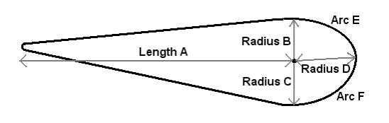
A Parameterised Wing Cross-Section.

Figure 2.7

The cell-growth method of shape optimisation uses an analogy with biological cellular growth to evolve suitable shapes. The cells are given ‘growth rules’ when they are created, and then when they develop according to those rules the resultant shapes are evaluated for their fitness values. The growth rules are treated as chromosomes and the search is performed using a GA to optimise the rules. Some dynamic feed-back during the growth process is possible using a variation on this approach which involves continually evaluating the developing shapes. If an area is suffering from very high stress for example, then more cells can be encouraged to grow in that area by adjusting the local growth parameters.

Primitive building blocks have been used by [Bentley 96] to evolve complex shapes using his Generic Evolutionary Design system. This system uses ‘clipped, stretched cuboids’ as the spatial partitioning representation and a GA performs the search by modifying genotypes which represent each individual design. This technique has enjoyed some great successes and has been used to evolve designs for tables, steps, heat sinks and many other components.

2.3.3 The voxel based approach to shape optimisation.

Previous work on shape optimisation has primarily concentrated around parametric representations of simple machineable shapes and has produced some very useful results [Smith 95a]. The parametric representation, which uses a series of parameters which are varied to alter the shape being represented, is a common choice for shape optimisation problems due to the simplicity with which restrictions on the shapes can be incorporated. As noted previously, unrestricted shape optimisation representations will frequently lead to ‘breaking’ the evaluation function and so parametric representations are often used to prevent this from happening.

This project uses a voxel based space representation which divides the shapes being optimised into a uniform grid of rectangles or boxes. Each subdivision is represented by a binary value which indicates whether the voxel is empty or full. Similar work has been done by [Chapman et al. 94] and [Shoenauer 95] however [Chapman et al. 94] used only standard GA operators and so suffered from the problems raised by [Watabe & Okino 93], and [Schoenauer 95] became concerned about the size of the chromosomes required to represent detailed or real-world problems and moved into alternative forms of problem representation.

Voxels may have any dimensionality, however representations of more than three dimensions are not required for the approach to shape optimisation taken here. Early experiments were performed in both one and two dimensions in order to explore the possibilities and gain insights into the problem area and the operation of the Genetic Algorithm.

The binary voxel representation leads naturally to very long chromosomes and the problems concomitant with the huge search spaces that they impose. However it also allows far more complex and varied shapes than a parametric representation - which is limited by the user’s choice of what aspects of the representation will be controlled through the parameters. In particular, holes in the material are entirely possible and even probable if there is a small low-stress area in a high-stress region - a parametric approach can only create holes where the user is expecting them to be required and has defined some appropriate ‘hole-control’ parameters to represent them.

Voxels are limited in that they can only form an approximation to a curve, however as the number of subdivisions used is increased, the approximation becomes more accurate and this can easily be controlled to suit the user’s accuracy requirements (Figure 2.8). There is a trade-off to be made in this situation however; the higher the number of subdivisions, the longer each individual evaluation will take. Thus the user must attempt to set the level of accuracy to be just sufficient if the amount of time taken by the analysis is also a consideration.

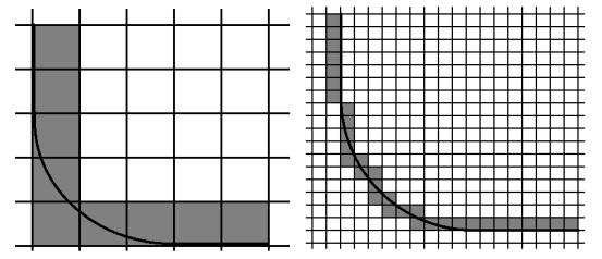
Lo-resolution Voxel Grid Hi-Resolution Voxel Grid

Figure 2.8

2.4 Miscellaneous relevant work on GA based shape optimisation.

[Watabe & Okino 93] describe shape design and optimisation by use of Free-Form Deformations (FFD) which use a matrix of control points to deform a default shape. This work includes three criticisms of a voxel based representation method for shape optimisation problems:

n Long chromosomes.

n Creation of small holes.

n Valid parents don’t often make valid children.

The crossover technique used in this work is to take a sub-set matrix of the control points and swap with the other parent. Three sets of experiments are described and the results are very good. The third set of experiments uses a Finite Element Method package in an attempt to minimise mass for a given maximum stress.

The paper: [Chapman et al. 94] covers genetic algorithms for shape optimisation under stress constraints. They use a one-point crossover claiming better results than from uniform crossover, a result which will be confirmed by the experiments detailed in Section 3.3.7. The work includes a simple rule for avoiding isolated pixels in the final representation by requiring a level of connectivity (4 directional) to a given ‘seed’ pixel, a concept which was adapted to the experiments performed here and extended to require two ‘seed’ voxels, one at each end of the voxel grid. They also assert that balancing a penalty parameter (for beams that fail the stress constraint) is critical for obtaining good results, as too high a penalty will produce beams that fall too far within the constraint (with the corresponding extra material this entails). This result is again confirmed by the experiments detailed in Section 3.3.4.

In [Bentley 96] a description of a very powerful generic shape optimisation tool is given. This system uses clipped, stretched cuboids as a primitive which is used to partition space into occupied/void areas. The results are very impressive and the system has developed designs for a large number of different parts and components. The emphasis is very much on the generality of the method, and it includes a technique which allows the user to easily specify the evaluation function from a library of already developed evaluation programs.

2.5 Conclusions.

This chapter has introduced the basic theories behind genetic algorithms, shape optimisation and stress analysis, and has described the problems to be addressed in later chapters. Previous work in this field has tended to concentrate on parametric representations and this has evolved good designs for aircraft wings and other components. The voxel based approaches to this problem have also been successful with work by both [Chapman et al. 94] and [Schoenauer 95] being done on a side-view beam topology optimisation problem with interesting results.

The rest of this thesis will describe the investigations undertaken on two separate problems from the field of shape optimisation using a voxel based representation and a modified GA to perform the search.

The first investigation will deal with an artificially simple example in order to experiment with GA operators with the intention of designing a selection of good, new, general purpose operators that perform well in a voxel based design space. The second investigation is intended to take those operators and the knowledge gained about the GA, and try to apply it to a real-world optimisation problem.

The operators designed and described in Chapter Three were also intended to be easily adaptable to a three-dimensional voxel representation, however this intention has yet to be proved.

This work will necessarily be restricted to just these two optimisations due to time limitations, however as the investigations have been successful, future work could extend the discoveries to virtually any two-dimensional shape optimisation problem which can be evaluated by a FEA package. This includes stress, loading, heat, liquid flow and electro-magnetic field optimisations.
Chapter Three.

Design and Testing of New Operators:

The techniques for the design of effective Genetic Algorithms are many and varied [Holland 75][Davis 91][Michalewicz 92] and a great deal of time can be spent adjusting parameters and trying different operators to obtain the most effective balance between convergence on a good solution and exploration of the problem domain. The stress analysis GA was initially used to evolve results for simplified versions of the problem area in order that the optimisations suggested by early results could be investigated rapidly. The simplified physics model of the beam’s stresses uses the mathematical approximations described in Section 2.3.1 in order to permit rapid calculation of the fitness of each individual in the population.

The work described in this chapter details early experiments with a one-dimensional chromosome followed by the extension of the experiments to two-dimensions and the subsequent GA optimisations. A comparison is then made between the results gained from the naïve GA and the results made possible following the addition of new operators.

3.1 The one dimensional experiments.

The first experiments were performed on a one-dimensional chromosomal representation of a beam cross-section. This very simple case was chosen as the starting point for the experiments as the expected results are well understood [Gere & Timoshenko 84] (pages 251-261) so it permits cross-checking of actual results gained against expected results. The programming involved in the Genetic Algorithm was not very complicated, and neither was the implementation of the simplified stress analysis physics model being used at this time, however it seemed reasonable to take this opportunity to verify their operation together.

The material and force parameters used for this initial set of runs were:

Area Represented = 0.75m²

Maximum Stress Allowed = 100 000 000 Pa (Steel)

Bending Moment = 200 000 Nm (Force applied)

The GA used settings of:

Mutation Rate = 0.005 (per bit)

Crossover Probability = 0.25 (per chromosome)

Population Size = 60

Ranking Pressure = 3

Chromosome Length = 64 bits

The mutation operator was the standard uniform mutation [Michalewicz 94] which flips bits in the chromosomes with each bit having an equal probability of being altered. The crossover operator used was also standard; the uniform crossover [Michalewicz 94] gives every bit in one parent’s chromosome a set probability of being swapped with the corresponding bit from the other parent. The GA used a roulette wheel selection mechanism with standard ranking (refer to [Whitley 89] for a good description of the most common selection mechanisms and their influence on diversity and convergence). An elitist mechanism was also implemented whereby the best solution found in any generation was guaranteed to survive unaltered into the next generation.

The fitness function described in Chapter Two as Equation 2.1 was designed to minimise the area of the beam cross-section (number of active voxels) whilst remaining capable of withstanding the maximum allowed stress, with a penalty value being applied to any solution which broke that strength constraint. A small additional factor was included in the fitness calculation based upon the maximum stress point in the beam. This has the effect of causing the valid solutions to continue to evolve towards the best possible solution (in this case a beam which minimises area and minimises the maximum amount of stress present).

A valid solution for this simplified model of the physics is any shape which does not exceed the maximum stress constraint, and the best solution would be the shape with minimal mass and the lowest value for its’ maximum stress point. For the purpose of this one-dimensional test virtually any shape at all will be valid. The row labelled `solution’ in Table 3.1 represents the number of generations taken to find a valid solution with the minimum required mass (mass-optimal).

Categories of solutions.

Figure 3.1

The best possible solution for this simple problem has all of the mass evenly divided with as much separation between the two areas as possible. By looking at the stress analysis equations in Section 2.3.1 it is clear that the further apart the two stress bearing components are, the lower the maximum stress encountered in the beam will be.

Ten trials of this program produced the results shown in Table 3.1. In each case a mass-optimal solution was found rapidly and then evolution continued towards the expected best solution for this problem (though it rarely found that solution during the period of the trial). Each trial was allowed to continue for 1000 generations (1000 Generations x 60 Population = 60000 Evaluations).

Trial	1	2	3	4	5	6	7	8	9	10
Solution	134	140	163	114	121	153	108	231	121	119
Best	-	-	-	464	-	-	-	905	-	-

Number of generations required to find solutions.

Table 3.1

These results show a mass-optimal solution being found after an average of 8424 evaluations, followed by a highly variable amount of time spent searching for the best possible solution. This is the type of behaviour expected from a Genetic Algorithm with a strong selection pressure for mass reduction and a much lower emphasis on optimality.

To confirm that the stress analysis mathematics was correctly implemented, the result of this particular problem was calculated independently, assuming that an ‘I’ beam is the best solution. For a steel beam 0.5m high the expected value for the second moment of area is approximately 0.001m⁴. Inspection of the variables generated by the stress analysis routine revealed a value of 0.00145m⁴ for the fittest member of the population when the chromosome represented a beam 0.516m high. This result indicates that the second moment of area is being calculated correctly and from this and Equation 2.2 it is clear that the stress calculations must also be correct.

Having determined that the GA and the mathematics involved in the stress analysis fitness function both work as desired, the experiments progressed to a more complex treatment of the problem; the representation of the beam cross-section was expanded to include two dimensions, vertical and horizontal.

3.2 A two-dimensional representation of a beam cross-section.

The one-dimensional representation was incapable of representing a complete ‘I’ beam and so made do with representing the top and bottom surfaces, omitting the vertical web from the calculations entirely. The two-dimensional representation is theoretically capable of representing the web, however the additional mathematics required to simulate the vertical and horizontal forces and calculate the stresses which necessitate the existence of a web are sufficiently complex that it would require the use of a finite-element method package. In order to maintain the advantages to optimisation available from extremely fast evaluations, it was decided to continue to use the same simplistic model of the physical forces applied to the one-dimensional problem and to treat the consequent absence of a properly designed web as an unavoidable side-effect.

The code modifications required to extend the beam cross-sectional representation to two dimensions were minor because the original representation was already dealing with the width of the beam, although as a single binary parameter which represented a whole line. The new representation used was a two-dimensional array of binary cells, a change that required the addition of an x component to the calculations finding the centroid of the shape. This simple change increased the size of the chromosomes from 64 bits to 32 x 64 = 2048 bits, creating a search space of 2²⁰⁴⁸ which is extremely large even for a GA.

Large search spaces can prove problematical for all forms of search unless they have an extremely simple solution space, for example: A problem with only a single well-defined optimum can be searched easily by even a simple technique such as hill-climbing. However most real-world problems are far more complicated than this and consequently increasing the size of the search area decreases the probability of the global optimum being found.

3.3 The GA experiments.

The following experiments were intended to improve the performance of the GA on a reasonably simple two-dimensional beam analysis problem in order that the optimisations discovered would be available for the more complex real-world analysis detailed in Chapter Four of this thesis. To try to ensure that the alterations and improvements made to the GA here will also prove beneficial to the real-world problem, it was decided not to concentrate on fine-tuning any of the various parameters available but rather to focus on the design and operation of various new operators. Parametric variations were restricted to an absolute minimum and were used only to determine the approximate values required to gain reasonable advantages from the new operators.

In the following experiments the following parameter settings remain constant unless mentioned otherwise:

Beam Dimensions = 0.05 x 0.10 metres

Bending Moment = 13000 Newton

Young’s Modulus = 2.0e8 Pascal

Voxel Grid = 32 x 64 voxels

3.3.1 Experiments using the naïve GA.

The first set of experiments with a 2D representation treated the chromosome as a long one-dimensional binary string which wrapped around at the vertical edges onto new lines to form the two-dimensional cross-section. The GA used a standard two-point crossover operator and the uniform mutation operator described in Section 2.2.3.
It used settings of:

Mutation Rate = 0.001 (per bit)

Crossover Probability = 0.35 (per chromosome)

Population Size = 20

Ranking Pressure = 3

Chromosome Length = 2048 bits

3.3.2 Results obtained from the naïve GA.

With this particular optimisation problem, the difficulty lay not in getting a valid solution, as even a solid beam will satisfy that requirement, but in getting a near optimal-mass solution. The first experiments were relatively unsuccessful in this regard, despite showing a tendency to evolve towards the same known best case found in the 1D trials, the results after 2000 generations were full of small holes and had extremely uneven inner edges. This can be seen in the typical end-of-run results shown in Figure 3.2 (the numbers represent the fitness values of each individual).

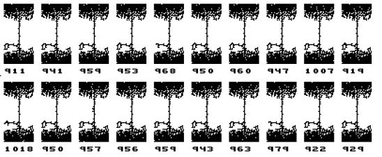
Typical End of Run Results From the Naïve Ga

Figure 3.2

The stresses were concentrated at the vertical extremes of the beam, so the material in the middle contributes less towards the total maximum stress that the beam can withstand than the material at the top and bottom. The GA even in this simple standard form rapidly removed material from the middle of the cross-section, and in the later stages of the experiments was observed to be moving material from low stress areas into high stress areas where holes were left near the extremities. However this first naïve GA approach took an extremely large number of evaluations in order to make significant progress, and this is not acceptable as later experiments will have a greatly increased evaluation time when the FE package is integrated. The rate of improvement was also seen to decrease as the run continued, levelling off to almost none at all by the end of the run. This means that the GA was not finding any further improvements to the chromosome, and as the results are visibly poor it indicates a general weakness in the operators being applied.

Figure 3.3 shows a graph of fitness values versus generation number for a typical selection of three of the ten trials performed with this program. The horizontal axis represents the generation number at which the results were found and the vertical axis represents the fitness values. Fitness values should be minimised for this optimisation, so the lower the fitness value, the better the quality of that individual solution.

The steepness of the curve during the first two hundred generations indicates that improvements were being made rapidly during this period, but as the optimisation approached the five-hundredth generation the rate of progress had diminished considerably. This effect was expected as the GA will rapidly find most of the obvious optimisations available and then the search will have to work harder to find any further worthwhile improvements. The problem with these results was that the naïve GA levelled off too early; the quality of solution at the end of the trial indicates that there were still many improvements to be made but the rate of improvement visible on the graph is almost zero.

Further work detailed in this chapter was therefore concentrated towards improving the operators and parameter settings for the GA, in order to achieve greater benefits during the early search period, and to produce better quality final results.

3.3.3 Experiments with the rank selection pressure.

This experiment was intended to discover the effect of changing the rank selection pressure variable used in the Genitor-type ranking algorithm [Whitley 89]. The pressure variable controls the proportional selection from the population based on the fitness ranked position within that population. A selection pressure of 1.0 results in a totally random selection (all members have equal probability of being selected), and higher selection pressures result in increasing probability that the fittest members of the population will be selected. The Genitor paper suggests that 1.5 is a suitable value to be used for many experiments, producing a good balance between population diversity and the rate of fitness improvements.

Implementation of the algorithm is exactly as given in the Genitor paper* :

linear_selection( pressure : float )

index = Population_size *

(pressure - Ö (pressure² - 4 * (pressure - 1) * random(1.0) ) ) / 2 / (pressure - 1)

The Genitor Linear_Selection() Function.

Figure 3.4

The population is sorted by its fitness values using a linked-list bubble-sort algorithm before the Genitor selection procedure is invoked, thus the result of the linear_selection() routine is an index to the linked-list, which in turn holds the position of the selected individual in the population.

The survivors selection procedure is simply to invoke this procedure once for every member of the population, each time copying the selected member of the old population into consecutive elements of the new population array.

The Genetic Algorithm used to perform the searches was the same as described in Section 2.2.3: ten trials were executed and the number of iterations per trial was set to 2000.

Figure 3.5 is a plot of the fitness of the best individual from the population averaged over all ten trial runs (on the vertical axis) against the generation number (on the horizontal axis). It shows the full set of results and clearly indicates that at selection pressures of 1.1 and even 1.3, there is insufficient differentiation between the poor members of the population and the fit ones. This results in chromosomes which violate the problem’s constraints being selected frequently enough to significantly degrade the average results. The large steps visible in both of these lines are caused by selection of individuals who are extremely unfit due to large constraint penalties being applied.

Figure 3.6 is a more detailed examination of the 1.3, 1.5, 1.7 and 1.9 selection pressures in which we see the expected results of higher pressures producing steeper fitness curves but ultimately resulting in similar overall fitness levels after 40000 evaluations. The 1.5 line is very slow to converge with the 1.7 and 1.9 lines, indicating that it takes significantly longer before it produces solutions of equivalent quality.

The very low selection values do not appear to cause enough selection pressure to avoid repeated constraint violations, although this may be affected by adjusting the Constraint Penalty Multiplier. The lower selection values also result in a slightly worse result after 2000 generations. As a consequence of these trials further experiments will be performed using a rank selection pressure of 1.7, as the suggested 1.5 is too close to the border-line where the constraints are being violated regularly and it also does not converge rapidly enough to the better solutions found at higher rank pressure levels.

3.3.4 Experiments with the constraint penalty multiplier.

The purpose of these experiments was to investigate the effects of changing the constraint penalty multiplier k used in the fitness function (Equation 2.1), and to find an appropriate value for this variable which maximises the search capabilities whilst avoiding an excess of non-viable solutions. The constraint penalty multiplier (hereafter referred to as the penalty value) is applied to the fitness value of any chromosome which has a maximum stress value greater than the constraint level, this will lower the relative fitness of that chromosome reducing it’s probability of survival into the next generation.

The penalty value is multiplied by the amount of stress which exceeds the stress constraint, so the effect on a chromosome’s fitness depends on the degree to which it is non-viable. This approach permits chromosomes which are only slightly over the constraint limit to survive for a while, thus increasing the population diversity at and around the stress constraint level.

The Genetic Algorithm used was as described in Section 2.2.3 except that the vertical web which runs through the middle of the ‘I’ beam was enforced after the operators were applied and before the evaluation function was called. Enforcing the web avoids the complicating issue of the amount of mass added by the web itself. A crooked web would contain more mass than a straight one, but the simple model of the physics being used for the evaluation stage does not contain any forces that would encourage a straight web. Rather than try to factor out the effect that the different randomly evolving webs would have on the final fitness values, it was considered to be more sensible to avoid the issue entirely in this way.

A population size of 20 and an initial run length of 1500 generations was used. The optimisation was performed ten times with each of the penalty values 1E-3, 5E-4, 1E-4, 5E-5 and 1E-5. Other parameters were set as follows:

Beam dimensions = 0.05m x 0.10m

Bending moment = 13000 Newton

Voxel grid size = 32 x 64 voxels

Crossover probability = 0.3 (per chromosome)

Mutation probability = 0.001 (per gene)

Rank selection pressure = 1.7

Stress constraint = 2.0e8 Pascal

The web was enforced.

The first results graph (Figure 3.7) for these trials shows a plot of the average fitness of the best individual from the population over the ten trials against the generation number. This graph is somewhat misleading as it indicates that as the penalty value is reduced the average fitness of the population tends to improve, unfortunately this is at the cost of increasingly poor solutions. What is not clear from this graph alone is that most of the fittest individuals at the lower penalty values are non-viable in that they break the constraint limit - often by a considerable amount.

The second graph (Figure 3.8) shows the maximum stress level of the best individual from the population averaged over the ten trials against the generation number, the stress limit constraint is marked as a horizontal line for reference. This graph clearly shows the difficulty with the lower penalty values - the data for 1E-5 is almost entirely above the constraint limit meaning that the majority of the solutions from the population were non-viable.

To be able to see the results for the 1E-3 and 1E-4 penalty values a considerable expansion of scale is required, Figure 3.9 shows the data from Figure 3.8 expanded about the constraint limit line (which is again included in the graph). Here even though the Maximum Stress average is very noisy data, we can see that the higher penalty values cause maximum stress to be further below the constraint limit than the lower penalties. The average for the penalty value 1E-4 actually crosses the constraint limit several times, but always returns to viable solutions after a short while.

Higher penalty values prevent recurrent violation of the stress constraint, but very high penalties reduce the available search space by forcing solutions to stay further within the limits. Even in the long trials the higher penalty values have this restrictive effect. This is in keeping with the results found by [Chapman et al. 94].

As the standard genetic algorithm verifies the viability of the initial population by using the fitness evaluation function (which incorporates the penalty value), the fitness/generation curves do not start at the same place for different trials but instead indicate that a lower average initial fitness can be achieved by using lower penalty values. This effect can be extremely useful, as a more fit initial population reduces the length of search required in order to achieve a given quality of result.

An ideal constraint penalty would allow the search to utilise the possibilities beyond the constraint limit at the beginning of the search and would cause more solutions to be valid as the search progresses towards it’s conclusion. This would encourage a fitter starting population, allow maximum population diversity initially and ensure that the eventual result population contains useful solutions.

These results suggest that a dynamically varying penalty value may result in more rapid optimisation in the early stages of the search whilst avoiding the problem of non-viable final solutions. This possibility was investigated and the results are included in the next section.

3.3.5 Experiments with a dynamically changing constraint penalty multiplier.

These experiments investigate the efficiency of using a dynamically changing constraint penalty multiplier rather than the static values used in the previous set of experiments. The rationale for this approach is that it may be good for the search if it is allowed to break the constraints during the early stages of the optimisation, but that the results at the end of the run must contain viable solutions.

The constraint penalty multiplier must start off low and increase as the optimisation continues, therefore the generation number will be used as the variable which controls the function:

f(generation) = constraint penalty multiplier

Equation 3.1

A linear function could be used to test this approach, however it is apparent that not only should the optimisation end with viable solutions, it should spend some time optimising the viable solutions before the end of the run. A more suitable curve function is:

constraint penalty multiplier = constraint base * ( 1.0 - e^{(- alpha * n)})

where n is the generation number.

Equation 3.2

This can be seen for several values of (alpha*n) in Figure 3.10 which shows the constraint penalty multiplier for each generation to fifteen hundred. The function describes a smooth curve from zero to a maximum, which is a proportion of the constraint base value determined by the value of alpha*n used. A higher value of alpha*n makes the curve more pronounced and results in a higher proportion of the constraint base value at the final generation.

The Genetic Algorithm used was as described in Section 2.2.3 with a population size of 20 and an initial run length of 1500 generations. The optimisation was performed ten times with each of the alpha*n values 0.5, 0.75, 1.0, 2.0 and 3.0.

The graph (Figure 3.11) shows the average fitness over ten trials for each of the tested alpha*n values plotted against the generation number. This graph shows the effect of very low constraint penalty multipliers in the first half of the run; the fitness curves go up from reasonable starting values to very poor results during the first four hundred generations, peaking at various points depending on the alpha*n value being used. It can be seen that the higher alpha*n values result in worse early results, but better results later on in the run, although the alpha*n = 0.75 line is anomalous in that it leads to a better final result than the 1.0 line.

The reason for the poor fitness values early in the run from higher alpha*n values is that the constraint penalty multiplier increases faster for the higher alpha*n values, thus the solutions are being penalised more strongly than those with lower values. The better final results appear to be due to the rapidly increasing penalty multiplier values forcing the search into a viable search space earlier, thereby giving the search more time to do fine-tuning on the final solution.

Comparing the fitness graph results with the data in Figure 3.12 which shows the maximum stress values over the same time period leads to some further insights into the behaviour of the fitness curves. The lower values of alpha*n lead to greater violations of the stress limit constraint, to the point where alpha*n = 0.5 doesn’t produce any viable solutions at all during the 1500 generations. Typically the higher values lead to viable solutions sooner, with the exception of alpha*n = 1.0 which takes longer to descend than alpha*n = 0.75. This can be seen more clearly in Figure 3.13 which shows a detailed view of the second half of the optimisation period and indicates that at alpha*n = 1.0 there were no viable solutions produced during the run.

Figure 3.13 shows that once the solutions enter the viable region by descending below the stress limit they rarely exceed that limit again, and indeed tend to remain at a fairly constant distance from the limit. This is possibly due to the constraint penalty multiplier value which, by continuing to increase, makes it less and less likely that a non-viable solution will be more fit than a viable one.

The fitness values at the end of the optimisation are not very much different than those obtained for good constant values for the constraint penalty multiplier. Table 3.2 contains the end of run fitness values for both constant penalty multipliers and the dynamic penalty multipliers, entries followed by a * are invalid solutions which exceeded the constraint penalty at the end of the run.

Constant constraint penalty multiplier values:

0.001	0.0005	0.0001	0.00005	0.00001
925.999	916.599	919.843	908.123	861.650 *

Dynamic constraint penalty alpha*n values:

0.5	0.75	1.0	2.0	3.0
1004.231 *	936.266	957.609 *	932.259	924.466

End of Run Values for Average Fitness.

Table 3.2

The intention of this approach was to allow maximum population diversity initially, but ensure that the eventual resultant population contains viable solutions, and in this regard the concept appears to be successful. As long as the alpha*n value is set to ensure a suitable constraint penalty multiplier value at the end of a run, the prevalence of invalid solutions in the early stages of the optimisation is not a problem for the type of problem being addressed here. This technique is obviously not suitable for optimisations of uncertain length or when the optimisation may be stopped before convergence and a viable solution will be required.

The fitness curve graph (Figure 3.11) shows that the eventual fitness of the best individuals varies very little, which indicates that the precise setting of the alpha*n value is not critical. However the evidence of both the fitness curves and the maximum stress curves is that a high value of alpha*n is better for the search, resulting in better final solutions and avoiding the danger of non-viable populations by a larger margin. Further experiments which use dynamically varying constraint penalty multipliers would have used an alpha*n value of 2.0, however, as it can be seen from the Table 3.2, the constant constraint penalty multipliers consistently perform better than the dynamic ones, therefore constant constraint penalty multipliers were used during the following experiments.

3.3.6 A new operator : smoothing.

The smoothing operator experiments were an attempt to directly address some of the weaknesses of the voxel representation by devising a new specialised operator which should aid the search by reducing the number of small holes and ragged edges produced by the GA. The new operator was intended to be capable of easy expansion from two-dimensions to n-dimensions in order that it would continue to be useful in the case of three- (or more) dimensional problems using the voxel representation. This would be an important issue for shape optimisations which are not capable of being represented by a simple cross-section, for example if a beam was to have a varying cross-section along its entire length then it would be necessary to represent it using three-dimensional voxels.

The GA parameters used were the same as the standard GA described in Section 2.2.3 and the new operator was applied in addition to the previous mutation and cross-over operators. The population size was set to twenty, and the number of generations was limited to fifteen hundred.

The new operator was designed to set a region of voxels to the average value of the previous contents of the voxels. Thus, if a region consisted primarily of ‘on’ voxels then the whole region would be set ‘on’ and similarly for ‘off’. This would achieve the desired results by filling isolated holes in solid regions, and would also eliminate the ragged edges where they overlap into the empty regions.

The size and location of the region to be affected was selected at random, however the size was restricted to a minimum of 2 voxels per dimension and a maximum of 1/4 of the dimensions of the voxel grid. These restrictions were imposed in an attempt to ensure that the smoothing operator would always have an effect when applied, and that the effect would not be to wipe out a huge area of the voxel grid. Because the location of the region was selected randomly, the operator was written in such a way that the region would ‘wrap-around’ to the opposite side of the voxel grid if it exceeded any of the grid’s boundaries.

In order to check the efficiency of the new operator, the modified GA was run ten times with each of the probabilities 0.0, 0.2, 0.4, 0.6, 0.8 and 1.0 of smoothing being applied on a per chromosome basis.

The results of the smoothing operator on the population can be seen in Figure 3.14 which plots the average fitness values of the best member of the population over the ten trial runs against the generation number, for each of the six different smoothing probabilities applied. This graph shows that the smoothing operator definitely increases the rate at which the fitness improves during the early part of the runs; the increased steepness of the curves and the generally lower final values at generation 1500 are good evidence that the operator is beneficial. There is some ‘ideal’ rate of application for this operator as witnessed by the improvement from 0.0 through to 0.6 and then the decrease in effectiveness from there to the 1.0 probability level. The best result from these trials was gained at 0.6 and so that will be the probability of smoothing used in further experiments.

Comparing Figure 3.15 which displays some typical end-of-run population members with the earlier results in Figure 3.2, shows just how effective this domain specific approach to operator design has been, especially at eliminating isolated holes and reducing ragged edges.

This set of experiments was intended to address two separate issues in operator design; firstly, will specially designed operators function as wanted when reducing particular undesirable effects during the optimisation process; secondly, can such operators be designed so that they can be expanded to n-dimensions with relative ease? The answer to both of these questions is a definitive ‘yes’. The rate of improvement in average fitness values and the increased quality of the final results produced using the new smoothing operator argues strongly for the first answer, and because the design of the operator relies on the geometry of the problem representation, the expansion to further dimensions should be extremely straight-forwards too.

The next two sets of experiments take the concept of n-dimensional operators further by attempting to formulate appropriate operators to replace the standard two-point cross-over and bit-wise mutation.

3.3.7 An n-dimensional crossover operator.

The two-point crossover operator which had been used up to this point treated the chromosome as a one-dimensional string of bits and therefore suffered from a problem with linkage - voxels which are adjacent in a two-dimensional grid are not necessarily adjacent in the one-dimensional string. This separation increases the possibility that useful building blocks (areas of the grid which contribute to a higher overall fitness evaluation) will be disrupted during the crossover procedure. The paper [Cartwright & Harris 93] describes the use of the UNBLOX crossover operator which was specifically designed to overcome these limitations with conventional two-point crossover. This operator swaps a rectangular area of the grid instead of the sub-string swapped by two-point crossover, if the area overlaps an edge of the grid then it is made to ‘wrap-around’ to the opposite side. The size and location of the area to be swapped are both selected at random, and in this implementation the area was restricted to a minimum size of two voxels per dimension in order that the operator would always have some effect when applied.

The crossover operators were used with the standard probability of 0.3 per chromosome and no changes were made to the standard algorithm or to any of the other parameter settings described in Section 2.2.3.

The graph in Figure 3.16 shows the results of ten trials using three alternative crossover operators, including the UNBLOX operator. The other two were the standard two-point crossover and another fairly common technique called uniform crossover [Michalewicz 92] which swaps genes between the two parents using a fifty percent probability for each individual gene to be swapped or left where it was. The horizontal axis again represents the generation from which the values were obtained and the vertical axis represents the average fitness of the best chromosomes from each of the ten trials at the end of each generation. The fitness axis scale has been adjusted to commence at a non-zero value in order to display greater separation between the three lines.

The results confirm that the UNBLOX operator does indeed perform better than either the two-point crossover or the uniform crossover techniques on this problem. The rate of descent of the UNBLOX line is quicker, indicating that the population converged to good solutions faster with this approach than with the other two, and the eventual end result after the fifteen hundred generations has a slightly better fitness value than those produced by the other techniques. The improvement was not as large as had been expected and after further thought it was realised that for this particular problem the optimal solution would be represented by a binary string consisting of a series of ones followed by a series of zeros, followed by another series of ones. This solution does not contain any inherently two dimensional features which would be destroyed by the two-point crossover, and so the UNBLOX operator only significantly improved the early stages of the search while the chromosomes were still converging towards the optimum.

The uniform crossover operator performed badly due its poor schema preservation qualities [Michalewicz 92][Holland 75], so it will not generally perform well on problems which rely heavily on solution sub-structures propagating through the population as the optimisation progresses.

UNBLOX is a useful crossover operator which consistently out-performs either two-point or uniform crossover on this problem, the work described by [Cartwright & Harris 93] seems to indicate that it can be used on other problems with similar results. Extension of the algorithm to further dimensions would be a simple matter and the arguments supporting its use on this two-dimensional problem also apply to voxel based representations of problems with more dimensions.

3.3.8 An n-dimensional mutation operator.

The standard mutation operator being applied to this problem relies on randomly flipping bits in order to permit the search to enter new areas of the solution surface. This approach does not apply any domain knowledge to the issues of mutation, and so it should be possible to get improved performance from the GA by designing mutation operators which directly address some of the perceived problems with the optimisation. These problems have been mentioned previously in Section 3.3.6 which discussed the smoothing operator.

A new mutation operator was designed which alters the contents of a randomly selected rectangular area of the voxel grid, it is referred to here as the ‘two dimensional’ operator. This operator can easily be modified to work in n-dimensions and works by affecting a relatively small area of the chromosome very intensively.

A second, somewhat altered version of this mutation operator was also designed and tested in these experiments called the ‘two by two’ area mutation operator. This operator uses a fixed mutation square of two by two voxels and was designed to be applied only if at least one voxel in the mutation area is already active. The theory behind this operator is that most of the modifications need to be made to the surface or interior of the evolving shape and that very little benefit will result from flipping isolated voxels in the middle of the void areas. The choice of a fixed two by two area was motivated by the observation that most of the irregularities on the surfaces would fit into such an area and that with only sixteen permutations possible (four binary bits), the probability of mutating a poor quality area into a more fit variation would be reasonably high.

The new operators were applied in addition to the original bitwise mutation operator, with a probability of 0.25 per chromosome of being applied. After each application there is a decreased probability of the same operator being applied again, with the probability of a further application being decreased to one half of its previous value each time. The experiments were performed ten times for each of the three alternative mutation combinations, over a period of fifteen hundred generations.

The graph in Figure 3.17 shows the effect of the two new mutation operators alongside the results obtained when neither of them was applied. The generation number is plotted along the horizontal axis and the average fitness of the best individual from the population at each generation is plotted vertically.

The addition of the two dimensional operator generally results in better performance than the bitwise operator alone, though the two lines do meet between generations 300 to 400. The steeper descent of the two dimensional operator line indicates that early performance was especially improved, and the final result after fifteen hundred generations is significantly better than previously. The two by two operator offers a similar rate of improvement during the early stages of the trial, a slightly better performance between generations 100 to 600 and finally converges with the two dimensional operator’s line at about generation 1000. This seems to indicate that although offering early benefits to the optimisation, it is not significantly better than the two dimensional operator in the long run.

In conclusion, two new mutation operators were designed with the particular intention of directly addressing the perceived problems with the prior optimisations. Both of the new operators were found to be more effective than the previous uninformed bitwise mutation, producing benefits to both the rate of early improvement and the final quality of solution generated.

In the absence of any other clearly distinguishing features, the two by two operator will be used during the further experiments as it offers a slight code speed advantage over the two dimensional mutation operator outlined above.

3.3.9 Dynamic mutation operator probabilities.

Dynamically varying operators have been used in many different studies of the GA, most relevantly [Tucson & Ross 96] who concluded that the applicability of this approach depends very much on the problem under consideration. The theory behind this approach is that some operators are more effective during a particular phase of the optimisation. For example, the smoothing operator described in Section 3.3.6 generally performs large scale changes to the chromosomes, and this makes it ideal for chopping away all of the excess material during the early stages of the optimisation. However towards the end of the optimisation, most of the changes which will improve the chromosomes are very small. This is due to the fact that the optimisation generally moves closer towards the problem constraints as it progresses and hence almost any large scale alteration is likely to cause a constraint violation.

Similarly the two by two mutation operator makes small changes in the chromosome, and while these are certainly very important during the early stages, they become the major source of progress when the population is close to convergence.

This experiment will use a dynamically varying mutation probability factor in the otherwise standard GA* to test this theory and see if any significant benefits can be achieved by this approach. The mutation probability will start at 0.5 and increase by 0.00025 per generation until it reaches a maximum of 0.8, which will occur after 1200 generations. The probability will stay at that level for the remaining 300 generations of the 1500 generation trial period. The starting value of 0.5 was chosen as it had been used in a previous experiment with the two by two mutation operator and had produced some good results. The ending value was set to 0.8 because it is sufficiently larger than 0.5 that the dynamic probability effects should be visible. The speed of 0.00025 was calculated after deciding that the mutation probability should stop changing before the end of the trial run.

The graph in Figure 3.18 shows the fitness curves for the static two by two mutation at a probability of 0.25 and the dynamic mutation probability. The vertical axis represents the fitness value versus the generation which is numbered horizontally. The two curves represent the average values of the best individual at each generation over the ten trial runs.

Figure 3.18 show that the static mutation operator starts off achieving better results and continues to do well right through the first 400 generations. It has the most significant advantage (over the dynamic probability) at approximately generation 310 where the two curves have their greatest vertical separation. From this point on the dynamic probability starts to catch up, and it achieves equal results near generation 800 when the dynamic probability value would have been:

0.5 + 0.00025 * 800 = 0.7.

The two curves cross and the dynamic probability continues to perform increasingly better until at the end of the trial run the dynamic probability average fitness was 861.399 compared with the static mutation’s average fitness value of 906.699.

On the basis of this experiment it appears that dynamic mutation probabilities have a positive effect on the efficiency of the optimisation. However the poor early results suggest that it may not work very well for short analyses or when the rate of early improvements is particularly critical. Following this result it was decided that the dynamic mutation probabilities would only be enabled when the experiments seem to need very high mutation rates towards the end of a run.

3.3.10 Comparison of modified GA with naïve GA.

After incorporating all of the most beneficial alterations and new operators discovered during the previous set of experiments the modified GA was run for ten trials of two-thousand generations in order to compare it’s results with those gained for the naïve GA earlier. The comparison can be seen in the graph Figure 3.19 which shows the fitness curve generated for the original GA and the same curve for the final modified GA.

The settings used to achieve these results were:

Population Size = 20

Ranking Pressure = 1.7

Crossover Probability = 0.35 (per chromosome)

Bitwise Mutation = 0.001 (per bit)

Two By Two Mutation Starting = 0.25 (per chromosome)

Two By Two Mutation Maximum = 0.75 (per chromosome)

Two By Two Mutation Speed = 0.00025 (per generation)

Smoothing Mutation Starting = 0.5 (per chromosome)

Smoothing Mutation Ending = 0.25 (per chromosome)

Smoothing Mutation Speed = -0.000125 (per generation)

The modified GA performs better than the original one throughout the optimisation period, with considerably better optimisations being found during the first ten generations and producing final results which are about 11% better than those found by the naïve GA. Also significant is the fact that the modified GA found almost no further improvements during the last thousand generations, the average best fitness over this time altered only from 846 to 838. Looking at the final results produced from this run in Figure 3.20, it is clear that they are very close to the theoretical global optimum for this problem.

3.4 Conclusions about the simplified physics model experiments.

The experiments described in this chapter were intended to find new operators and better parameter settings for a naïve GA, thereby improving it’s performance ready for application to a complicated real-world problem. The focus has not been on fine-tuning the parameter settings for this particular optimisation, but rather on determining the effects of the various parameters. Similarly the new operators were not designed to solve the unique difficulties uncovered by the experiments, but to address issues relating to a generalised n-dimensional voxel based representation.

The results have shown that although a naïve GA does indeed suffer from the problems suggested by [Watabe & Okino 93], a small selection of operators informed only by domain knowledge about the representation, will effectively solve each of these difficulties and permit the production of useful results.

The final system uses a normal bitwise mutation operator in addition to the two new mutation operators, smoothing and two by two. Both of the new mutation operators are applied using a time-varying probability in order to maximise their effects at the appropriate stages of the optimisation. The smoothing operator rapidly cuts away unwanted areas of material during the early stages of the optimisation and can help to smooth ragged edges and fill small holes later on. The two by two mutation operator is highly effective at both smoothing off ragged edges and at filling in small holes in the material if they occur in undesirable places. The two-point crossover operator has been replaced by the n-dimensional UNBLOX operator described in work by [Cartwright & Harris 93], and this alteration directly answers the issue of whether the children produced by crossover will be valid with any degree of reliability. Finally the Genitor style ranked survivor selection [Whitley 89] permits easy control over the degree of exploitation versus exploration that occurs, and also separates the proportion of fit individuals selected from their actual fitness values, making the whole GA less sensitive to changes in the type of evaluation function being applied.
Chapter Four.

Transferring the solutions to real problems.

The motivation for the experiments detailed in Chapter Three was to produce an effective GA which can quickly and efficiently optimise a two-dimensional shape optimisation problem represented by a voxel grid. The work so far has used an evaluation function based on a highly simplified physics model of the forces and stresses involved in a beam loading problem. The experiments in this chapter will detail how the same improved GA was then modified to use a commercial Finite Element Analysis (FEA) package called Ansys* as it’s evaluation function, and how the combination of the optimised GA and Ansys worked to optimise an annulus design problem which has been under research by Rolls Royce. It will be seen that although several major difficulties were encountered in both the inter-package communications and in the optimisation itself, the difficulties were not insurmountable and the final system was capable of producing both interesting and useful results.

4.1 Motivation for this approach.

There were several different motivations for taking this approach to extending the experiments. It was considered important to ensure that the arguments put forwards in Section 3.3 were correct and that the optimisations made to the GA would still be applicable to a much harder real-world problem. Engineers do need to solve this type of shape optimisation problem and if this approach is successful then it could assist them to achieve better results. GA optimisations can easily be modified into hybrid systems [Tucson et al. 97] and in this case the computer would rely on an engineer’s practical experience and knowledge of the problem domain to direct key choices in the optimisation process. Finally, GAs are also an ideal tool with which to address this type of problem, as the population of final solutions will allow engineers to choose the one they consider most appropriate using any further criteria which were not built into the fitness function.

4.2 The annulus design problem.

The annulus design problem comes from a specification supplied by Rolls Royce plc to Richard Smith during his time in the Mechanical Engineering Department at Edinburgh University. The full original specification of this problem is included as Appendix A. The problem is to design an annulus which is to function as the hub of a jet-engine turbine propeller. This part will be subject to extreme forces due to its high speed of rotation and the attachment of the turbine blades to its outer circumference.

The actual optimisation assumes that the part is axisymmetrical around the axis of rotation, and consequently it reduces to the two-dimensional shape optimisation problem shown as Figure 4.1.

Annulus Axisymmetric Cross-section.

Figure 4.1

The optimisation as performed for these experiments involved reducing the mass of the annulus whilst observing a series of four separate stress constraints. The constraints relate to the hoop stresses at the inner and outer circumferences and the radial stresses along the centre line of the annulus from the hub to the rim. Hoop stresses are those that go around the annulus, effectively into and out of the page given the cross-sectional picture in Figure 4.1. Radial stresses are those which go from the hub to the rim (or vice-versa) or left and right in Figure 4.1.

4.3 Implementation details.

The GA fitness function was defined as:

fit = -weight[b] + (1.0 / total_stress)

Equation 4.1

Constraint penalties were applied if any of the four constraints limits were broken, and the constraints were ordered in importance by using 4*K* for the most important, 3*K for the second most important, 2*K for the next and 1*K for the least important constraint.

In order to allow the GA program to use Ansys as its evaluation function, it was first necessary to find some way of communicating data about the shape to be optimised and the final evaluation value between the two programs. The Ansys manuals describe a method whereby it should be possible to link the entire Ansys program into a user supplied program as a library, however this relies on the use of a Fortran compiler and for the PC compatible version of Ansys it would need to be a Windows™ Fortran compiler. This approach was problematical due to the difficulties involved in getting a suitable compiler and because the GA as written and optimised so far was entirely written in C.

An alternative method of communication was attempted whereby the GA program would ‘call-out’ to Ansys using command line specifiers to control the Ansys program. It would also read and interpret the files that Ansys writes to preserve the results of an evaluation. This method was implemented and worked satisfactorily for very small problems, however the ‘call-out’ made use of the C ‘system()’ command which in turn uses a DOS™ type command box in order to interpret the command specified. This resulted in very slow evaluations as the DOS box takes two seconds (per evaluation) to open, and also permitted a memory leak from either the Windows DOS box or the Ansys program to gradually use up all available system resources which would eventually cause a crash after approximately ten generations with a population of twenty individuals.

After detailed study of the Ansys ‘Programmer’s Manual’ a third alternative was discovered which involved the use of the Ansys internal macro programming language. This macro language whilst insufficiently powerful for the implementation of the full GA, does include instructions which perform counted loops and can ‘call-out’ to other programs. A memory leak problem was anticipated with the ‘call-out’ function, however by changing the orientation of the optimisation in this way, the ‘call-out’ would only be necessary once per generation instead of once per individual evaluation. Therefore if the memory leak was from the DOS box the program could reasonably expect to evaluate twenty times as many generations before crashing from the leak, which might be acceptable if no data is lost when the program stops. The reduced frequency of ‘call-outs’ also meant that the speed lost due to the start-up time for the DOS box would not be such a problem.

A simple macro was devised which looped a user-specified number of times and performed a ‘call-out’ to a small C program on each iteration. This worked extremely well, and did not suffer from memory leak problems even after one-thousand iterations. The memory leak was therefore in Ansys itself, which would not be a problem as the new approach only involves starting Ansys once and then permitting the macro to control the optimisation process.

Ansys requires two different data files in order to define the shape which it is attempting to optimise; the nodal position file and the element connection file. The nodal position file specifies where in the optimisation space the nodal points are located. Each node has a number which is used in the element connection file to specify which nodes are connected together to form elements. Connected nodes form the corners of the voxels which combine to form the shape to be optimised. Figure 4.2 shows how these files combine to define the optimisation shape. The nodes are represented by the circles, and the lines represent the connections between them. In this implementation, the node position file is constant which allows it to be set up during the initialisation phase and thereby saves valuable processor time. The element files are created from the chromosomes just before the GA program releases control back to the Ansys macro.

Nodes are Connected Together to Form Elements.

Figure 4.2

Interpreting the files required by Ansys was achieved by detailed reference to the Programmer’s manual and cross-checking with the output produced from a very simple analysis performed on a fully occupied rectilinear grid. The appropriate routines were added to the existing GA code and a command-line interpreting capability was also added so that the Ansys macro could easily command the GA program to initialise the population or produce the next generation, as appropriate. Other functions added to the GA code included the ability to convert the chromosomes into the representation expected by the Ansys program and write these out in a series of standard files used by the macro. With these modifications in place the evaluation macro which would control the Ansys evaluations was written.

A listing of the full Ansys macro can be found in Appendix B as Listing B.1 followed by an abbreviated macro which was originally used to check that the evaluation would perform as desired. This abbreviated macro, included as Listing B.2, performs the following operations:

n Set the evaluation mode to Batch processing

n Restrict the amount of excess data that Ansys produces to an absolute minimum

n Instruct Ansys to output data about the stresses produced

n Set up the properties of the materials to be used

n Establish the element types to be used to represent the voxels

n Read the file specifying the locations of all of the corner point nodes

n Define the type of analysis to be performed

n Specify the rotation speed of the annulus

n Set the level of accuracy of analysis required

n Read the file specifying the nodal connections which form the voxel elements

n Select a subset of the nodes defining the extreme right-hand edge of the annulus

n Apply the force which simulates the attachment of the turbine blades

n Instruct Ansys to perform the evaluation

n Output the relevant results for both Bore and Hoop stresses to standard files

n Exit

The complete analysis macro commences by calling the GA program (called ‘stress.exe’) with command line options to initialise the population. It encloses the above evaluation commands with a loop that iterates a user specified number of times, calling the GA program at the end of each loop in order to generate the next generation of chromosomes. Due to restrictions in the macro language it was not possible to construct suitable filenames for the output files for each individual member of the population, so the analysis portion of the macro was simply repeated twenty times inside the loop with a different set of filenames for each repetition. This obviously fixes the population size to twenty individuals, however the GA program is capable of modifying the macro instruction file before the analysis commences. This permits a simple addition to the program to create the appropriate number of evaluation instructions if a variable population size is desired.

4.4 Results from the basic system.

The purpose of these first experiments was to determine if the Ansys macro-language/GA hybrid system would work as intended and also to see how well it performs on the annulus optimisation problem.

The settings used for the GA were:

population size = 20

cross-over rate = 0.3

mutation rate = 0.8

smoothing rate = 0.8

rank selection pressure = 1.7

horizontal size of area = 62 voxels

vertical size of area = 27 voxels

constraint penalty = 0.00005

The settings used for the annulus were:

horizontal size of area = 0.25 metres

vertical size of area = 0.05 metres

radius of hole = 0.10 metres

blade force = 10e5 Newton/radian

Young’s modulus = 2.238e11 Pascal

material density = 8.221e3 kg/m³

revolution speed = 1571.0 radian/second

The constraints to be observed were:

hub hoop stress < 1330 MPa

rim hoop stress < 396 MPa

inner radial stress < 741 MPa

outer radial stress < 334 MPa

The basic system was applied without further modifications to the annulus optimisation, however the problem as specified by Rolls Royce is extremely tightly constrained which meant that the attempts to solve this problem using random population initialisation violated all of the stress constraints by large amounts, and the rate of improvement in the population, when extrapolated beyond the time period allocated to the experiments, indicated that a valid solution would not be found for some considerable number of generations still to come.

To circumvent this problem the population was instead initialised with a selection of variations on the annulus design supplied by Rolls Royce, which were modified further by an intensive random mutation operator which added and removed small areas of material over the surface of the annulus design. This kind of intelligent initialisation is reasonable as a user will often want to start the GA with the existing designs in order to see what improvements can be made. Even when a totally new shape is being designed, the user will normally have some expectation about the final form, and this could be drawn by hand and scanned into the program. The intelligent initialisation approach meant that the initial population was not unreasonably far outside of the stress constraints, yet supplied the optimisation with sufficient variation that the population did not rapidly converge onto a single solution. Some of the results from this basic system can be seen in Figure 4.3 which shows six members of the population after seventy-five generations.

Results of the Basic Annulus Optimisation After 75 Generations.

Figure 4.3

The results shown in Figure 4.3 are extremely poor, the lack of symmetry around the horizontal axis and the uneven surfaces are just the most visible failings in this set of results. Another problem which becomes visible when using Ansys to analyse an individual was that extremely high stress values were present in the corners of many of the voxel areas.

The graph shown as Figure 4.4 shows the fitness curve for these results, with the generation represented on the horizontal axis and the fitness value of the best

individual of the population shown as the vertical axis. Due to the fact that the fitness values returned by this evaluation are negative, the curve is vertically inverted compared with the curves produced for Chapter Three.

Although the first thirty-five generations show a substantial rate of improvement this is mainly due to the violations of the stress constraint becoming less severe. At the fifty-second generation the first valid solution is found and the curve from there on is almost level, indicating that no further significant improvements were found. The graph indicates that the GA is performing the optimisation correctly and is capable of producing a valid solution when supplied with an initial population that breaks the stress constraints, however it also shows that the rate of optimisation is very poor.

The results of this initial experiment are only moderately encouraging; without any special operators being designed for the new problem domain, the GA has managed to take a population of poor annulus designs and improve them. The first stage in this process was to obtain a viable solution, and the GA achieved this during the first fifty-two generations. The second stage should involve improving the solution to try to find a near-optimal answer, but the GA only managed to improve the fitness value from -108.245 at generation 52 to -107.156 at generation 75.

A further investigation into the reasons for this failure was made, and the fitness log file produced during the optimisation was examined to try to find an explanation. The log file is included in Appendix C as Listing C.1 and it is clear from the predominance of extremely large negative numbers in the final twenty generations that the majority of the population is violating at least one and probably several of the stress constraints. This indicates that the stress constraints are so tight that even minor changes to a valid chromosome can result in extreme violations of them.

The experiments with the basic system operating on the annulus problem have highlighted several major problems which the optimisation must overcome in order to be successful:

n Random initialisation of the population was found to produce results that violated all of the constraints so badly that it would take a very long run just to get a valid solution.

n It takes a very long time to find a valid solution even when initialised with reasonable designs.

n Valid solutions when found contained small holes and protuberances and were not symmetrical.

n The constraints imposed are extremely tight and cause a proliferation of invalid solutions from even small changes in the chromosome.

n Extremely high stress values for both hoop and radial stresses are present in the corners of many of the voxel areas.

These problems are addressed in Section 4.5.

4.5 Improvements made to the system.

In order to improve the efficiency of the optimisation process several improvements were made to the GA and to the form of the analysis. Firstly, in order to reduce the search space of the problem being optimised, a symmetry constraint was imposed, with the axis of reflection defined to be horizontal through the middle of the shape. The GA was modified to reconstruct the final shape in its entirety only when producing the element definition files to be accessed by Ansys. This simple modification reduces the search space from a typical size of 2²⁵⁴² for a 62 voxel by 41 voxel grid, to 2¹³⁰² which represents a 62 voxel by 21 voxel half-grid. The centre line along the axis of symmetry is not mirrored as it is now enforced by the GA to be always turned on. This also provides a guaranteed central line of elements for the stress measurements to be taken from.

One of the problems that was highlighted in the first set of experiments is that the FE package does not deal very well with sharp corners. This is a general failing in FE packages and not a particular weakness of Ansys, but it constitutes a very major problem given the use of a voxel based representation. In an attempt to alleviate this problem a second type of element was defined by the optimisation macro. The new element type is triangular and is created by specifying connections between groups of three nodes in the element connection file. These triangular elements are added to the shape at all suitable ‘steps’, which are identified by convolving the voxels in the shape against a series of four matching template masks . If each square in the mask matches the value of the voxels surrounding an empty voxel then the appropriate triangular element is created in the ‘step’. The convolution masks and the triangles which they cause to be inserted are shown in Figure 4.5.

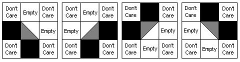
Convolution Masks for Triangle Insertion Process.

Figure 4.5

The triangular elements were applied in order to smooth off the corners left at voxel ‘steps’, so it was expected that the artificially high stress levels reported by the FE evaluation at the corners of the voxel areas would be removed.

The small holes appearing in the material may be due to one or more of several different causes:

n The holes are appearing in low stress areas and are a valid part of the solution.

n They are caused by the mutation operators and would be removed if the optimisation was allowed to progress further.

n They are an attempt by the GA to represent a lower density material indicating that although material is needed at that location, it need not be as strong as the basic material being used.

Regardless of which of these explanations is accepted, the reality is that current manufacturing processes would find it extremely difficult to produce a solid annulus with these small holes present, so it is therefore desirable to modify the operators to try to eliminate them, or at least reduce the number of them present. This was accomplished very easily by modifying the two by two mutation operator (the operator which can either fix holes or cause them to appear) to only mutate areas where, as well as at least one voxel being turned on, at least one of the four voxels is also turned off. The result of this modification is that the two by two mutation operator can now only mutate at the boundaries of the shapes being formed, and consequently it should also help reduce the number of small protuberances.

The improved GA for annulus optimisation used the same settings as the basic system for all parameters except that the chromosomal grid was set to 21 voxels high, which is mirrored due to the symmetry constraint to produce a voxel grid height of 41 voxels.

The analysis was permitted to continue for 114 generations and this took approximately twenty-four hours in total. The fitness curve for this analysis is shown as Figure 4.6 which shows the generation number on the horizontal axis and fitness on the vertical axis, the data line represents the fitness of the best member of the population at each generation. This graph shows a considerable improvement in the GA performance over the basic system. The population once again starts without

any valid individuals but some extremely rapid early improvements followed by regular small advancements generate the first valid member after only thirty-one passes. Once again the GA has difficulty improving upon this first valid individual, however examining the detail of the portion of the graph where valid individuals were created (Figure 4.7) reveals constant small improvements being made with occasional larger changes. The fitness log for this run is included in Appendix C as Listing C.2.

Some of the final population created by the improved GA is shown in Figure 4.8 which displays three of the twenty individuals and shows a clear improvement in quality over the results generated previously. The small protuberances have been totally eliminated and only a few members of the population contain small holes. The rate at which a valid solution was found is considerably faster than the basic implementation, and once found, the GA continued to improve upon this solution even to the very last pass of this trial.

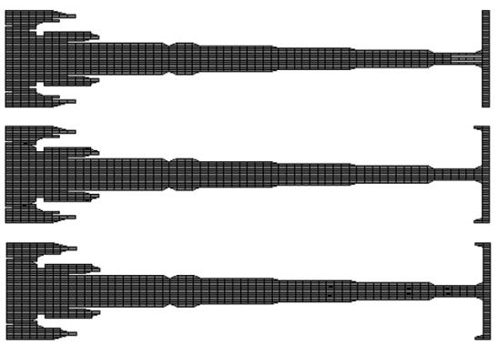
Final Annulus Cross-Sections From Improved GA

Figure 4.8

After using Ansys to examine the solutions produced by this optimisation, it was possible to confirm that the triangles are indeed working as expected and the amount of stress in the regions immediately surrounding a step which has been smoothed is far less than for the steps which have not been smoothed. Figure 4.9 shows the stress values calculated by Ansys for the voxels surrounding steps in two typical runs and clearly shows how the triangles permit the excess stress to be distributed in a more even pattern. Darker shades indicate higher stress levels in both of these pictures.

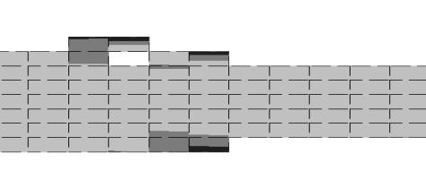
Without Smoothing Triangles.

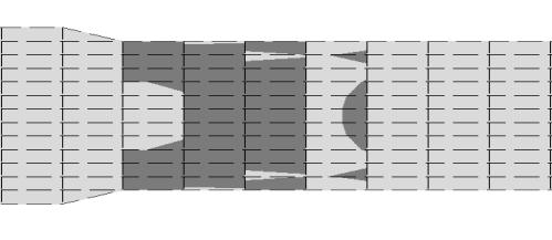
With Smoothing Triangles.

Figure 4.9

Examination of the final results of these experiments reveals several unexpected features, in particular the overhanging component in the cob of the annulus is extremely interesting. A trial analysis using Ansys to evaluate the shape with the overhang replaced with a more conventional sloping solid cob resulted in violations of both the maximum radial stress constraint and the inner hoop stress constraint. Several different adjustments were made but the violations could not be easily repaired. These results imply that the overhang is a genuine benefit to the annulus design, permitting a lower mass solution than is possible without it’s presence. A parametric representation of the annulus would probably not have discovered this result because there is no obvious reason to suspect that an overhang will be beneficial, and so there would be no incentive to provide variable parameters which would allow the overhang to form. This unexpected discovery thoroughly vindicates the choice of a voxel representation, and validates the points made in Section 2.3.3

Another interesting result is the presence in the best individual of the population of two short horizontal holes near the point where the neck of the annulus connects to the rim. This is unexpected as the operators have been heavily biased against producing such holes which implies that they too offer genuine advantages to the annulus design. The holes appeared just before the end of the trial run and it would be interesting to see if they remain after many further generations or whether they are just fore-runners of some larger change in the shape.

4.6 Conclusions about the real-world system.

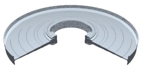
The Best Annulus Design From the Final Set of Experiments

Figure 4.10

This Chapter has described the experiments which extended the work from Chapter Three to deal with a real-world problem using a full commercial Finite Element Analysis package.

Two sets of experiments were performed: the first set took all of the previous work and applied it directly to the new problem domain. As was expected, this was not very successful due to problems with population initialisation, holes and protuberances, lack of symmetry and extremely high stress values due to the sharp corners caused by the voxel representation.

The next set of experiments applied the same principle of directly addressing the problems that was used successfully in Chapter Three, this time via operator modifications and additions to the representation used. These experiments were considerably more successful, providing much faster early improvements leading to valid individuals very quickly. The rate of further improvements after discovery of a valid individual was also much greater which lead to continual progress throughout the whole optimisation run.

The final results gained from the improved optimisation process contained several interesting features and should be viable annulus designs according to the stress figures produced by Ansys.

Chapter Five.

Conclusion:

The work described in this thesis was intended to find a set of suitable operators to permit effective optimisation of a voxel based representation using an evolutionary algorithm. The experiments then attempted to discover whether the combination of the GA coupled with the voxel based shape representation could perform a real-world analysis task with worthwhile results.

5.1 Summary of Conclusions.

The choice of a voxel based representation for this problem was contrary to some of the arguments in the literature [Watabe & Okino 93], but the results showed that with a combination of good operator design and a careful, principled and informed choice of the domain knowledge to be applied, the problems of small holes, long chromosomes, meaningless crossover and uneven edges can be avoided. The advantages to be gained from the voxel representation make the additional effort required to get good solutions a worthwhile endeavour.

The experiments which were performed on the beam cross-section optimisation were evaluated by a fitness function which makes simplifying assumptions about the physics of the situation in order to permit rapid investigations into the design and implementation of better operators. They included: implementation of the Genitor rank selection algorithm due to [Whitley 89]; discovering the effect of changing the constraint penalty multiplier; experimenting with a dynamically changing constraint penalty multiplier; development of the new mutation operator called ‘smoothing’; implementation of the UNBLOX crossover algorithm [Cartwright & Harris 93]; creation of another new mutation operator called ‘two by two mutation’ and experimentation with dynamically changing mutation probabilities. These experiments resulted in considerable improvements in the effectiveness of the GA at searching for solutions to the beam optimisation problem, eventually reaching the point where the GA was finding a near optimal solution in less than a thousand generations (Section 3.3.10).

The annulus design experiments used the knowledge gained from this first stage of operator design and testing, and applied it to the real-world problem of optimisation of a turbine annulus for minimum mass within multiple stress constraints, using the Ansys commercial FE analysis package to perform the evaluations. These experiments were quite unsuccessful initially, with very poor results being generated and several difficulties with the interactions between voxels and the FE package being discovered. However, using the knowledge about the GA gained during the beam analysis and by directly addressing the problems as they manifested themselves in the voxel grid, it was possible to solve these difficulties and achieve a successful optimisation system. The final system was able to optimise an annulus design which initially failed several of the stress constraints and was quite heavy, into a light-weight annulus which met all of the constraints.

One of the key issues involved in taking an approach that involved two separate optimisation stages, was whether the operators designed for the simple beam optimisation problem would work effectively on a much harder problem like the annulus design? The results gained from the annulus design experiments seem to indicate that this is the case, which is an important result for researchers who are dealing with similar long evaluation period GAs and who may wish to design operators in a more interactive way.

A very important result was gained from the final set of annulus design experiments; the generation of an annulus with an overhanging ledge in the cob was totally unexpected and argues strongly for the use of unbounded representational approaches such as voxels. It is highly unlikely that a person designing a parametric representation for the annulus optimisation would include parameters to represent such a ledge, unless they already expected that it would be required.

The real-world optimisation system used to evolve an annulus design was not directed towards that problem in particular. By modifying the macro which controls Ansys it should be possible to use the same system to evolve designs for many different two-dimensional components, provided that Ansys is capable of evaluating the fitness of the individuals. The restriction to two-dimensions is not necessary either, however no work was done using these operators on a three-dimensional optimisation so it is not known whether they will work as desired (although it would appear to be likely).

5.2 Further work.

Further developments and improvements to this optimisation program should address the weaknesses of the system as it stands, some simple code additions should also be mentioned. These will now be considered in turn:

1. The GA requires a better means of initialising the population to a prepared design shape. It should be a relatively easy step to add code that will take a scanned image of a design and allow the user to clean it up and use it for initialisation of the population. Such a modification would simplify the incorporation of preconceived solutions into the design space, and would also be extremely useful for design modifications if the program was developed into a hybrid system.

2. The system has not yet been tested on three-dimensional problems and no experiments have yet been performed to test the effectiveness of the n-dimensional operators in more than two-dimensions. The key issue in such experiments would be to see if the operators do extend to three-dimensions as easily and effectively as was predicted in Chapter Three.

3. The major weakness of the voxel representation was not due to the long chromosomes or any of the other predicted problem areas. Rather it was due to the fact that finite element analyses do not deal very well with the sharp corners or the voxels. It may be possible to rewrite the Ansys macro to use the 'auto-meshing' capabilities of the package; auto-meshing permits the Ansys program to subdivide the outline of a shape into suitable elements for analysis itself. This approach would involve a further change of representation from voxels to the auto-meshed outline of the shape under consideration, but this should be irrelevant as the two representations would be functionally equivalent.

4. Finally, on a technical note, the optimisation fails after a large number of generations due to the creation and constant expansion of a ‘page’ file maintained by Ansys. It would aid both the execution speed and the usefulness of the system if some way of preventing its’ growth or destroying this file between generations could be found.

In summary, with only a few modifications to the GA program, it should be possible to allow this system to use human input and create a hybrid system which will work with an engineer present to assist in the design process. Such systems are becoming increasingly popular as they combine the search power of a GA with the knowledge and design intuition of experienced engineers [Tucson et al. 97].

Appendix A - Rolls Royce disc optimisation problem specification (ref. E/ASS/40002) is available from the author or from Dr. F. Mills at Dept. of Mechanical Engineering, Edinburgh University.

Appendix B Ansys macro listings

Listing B.1: Full optimisation macro mask listing

This appendix contains the macro mask that is used to build the input file to Ansys to perform the full optimisation.

/batch !put Ansys into batch processing mode

/uis,msgpop,3 !limit the number of warning messages produced

/prep7 !enter the pre-processor mode

/nolist

/nopr

/nop !turn off most of the text file outputs

outres,all,none

outres,strs,last !set the output mode to dump stresses only

time,1 !set the time stage for the optimisation to occur at

uimp,1,ex,,,**** !mask statement for the material properties

uimp,1,dens,,,**** !mask statement for the material density

et,1,plane42,0,0,1,,2,0 !element type 1 is rectangles

et,2,plane2,,,1,,2,0 !element type 2 is squares

finish

/syp,"f:\stress",1 !make the stress.exe program initialise the population

/prep7

nread,nodes,dat,f:\ !read in the node position data file

antype,STATIC !specify the type of analysis to be performed

omega,0,****,0,0 !mask statement to set the rotational velocity

eqslv,iter,1e-005,0 !set the equation solver limits of accuracy

finish

*do,pass,0,loops,1 !for a user specified number of loops do

/prep7

numcmp,elem !compress the element numbers down to start from 1

eread,elems00,dat,f:\ !read the element connection file

nsel,s,loc,x,****,**** !mask statement to select the rightmost column of nodes

f,all,fx,**** !mask statement to apply the blade load force to selected nodes

nsel,all !select all nodes again

/solv

solve !solve the analysis

/post1

/output,xsol_00,log,f:\ !specify the output file

etable,table,s,x !dump the radial stresses into the output file

pretab,table

/output,zsol_00,log,f:\ !specify the output file

etable,table,s,z !dump the hoop stresses into the output file

pretab,table

/output

finish !finish output processing mode

/prep7 !do it all again for the next 19 members of the population…

esel,all

edele,all

numcmp,elem

eread,elems01,dat,f:\

nsel,s,loc,x,****,****

f,all,fx,****

nsel,all

/solv

solve

/post1

/output,xsol_01,log,f:\

etable,table,s,x

pretab,table

/output,zsol_01,log,f:\

etable,table,s,z

pretab,table

/output

finish

/prep7

esel,all

edele,all

numcmp,elem

eread,elems02,dat,f:\

nsel,s,loc,x,****,****

f,all,fx,****

nsel,all

/solv

solve

/post1

/output,xsol_02,log,f:\

etable,table,s,x

pretab,table

/output,zsol_02,log,f:\

etable,table,s,z

pretab,table

/output

finish

/prep7

esel,all

edele,all

numcmp,elem

eread,elems03,dat,f:\

nsel,s,loc,x,****,****

f,all,fx,****

nsel,all

/solv

solve

/post1

/output,xsol_03,log,f:\

etable,table,s,x

pretab,table

/output,zsol_03,log,f:\

etable,table,s,z

pretab,table

/output

finish

/prep7

esel,all

edele,all

numcmp,elem

eread,elems04,dat,f:\

nsel,s,loc,x,****,****

f,all,fx,****

nsel,all

/solv

solve

/post1

/output,xsol_04,log,f:\

etable,table,s,x

pretab,table

/output,zsol_04,log,f:\

etable,table,s,z

pretab,table

/output

finish

/prep7

esel,all

edele,all

numcmp,elem

eread,elems05,dat,f:\

nsel,s,loc,x,****,****

f,all,fx,****

nsel,all

/solv

solve

/post1

/output,xsol_05,log,f:\

etable,table,s,x

pretab,table

/output,zsol_05,log,f:\

etable,table,s,z

pretab,table

/output

finish

/prep7

esel,all

edele,all

numcmp,elem

eread,elems06,dat,f:\

nsel,s,loc,x,****,****

f,all,fx,****

nsel,all

/solv

solve

/post1

/output,xsol_06,log,f:\

etable,table,s,x

pretab,table

/output,zsol_06,log,f:\

etable,table,s,z

pretab,table

/output

finish

/prep7

esel,all

edele,all

numcmp,elem

eread,elems07,dat,f:\

nsel,s,loc,x,****,****

f,all,fx,****

nsel,all

/solv

solve

/post1

/output,xsol_07,log,f:\

etable,table,s,x

pretab,table

/output,zsol_07,log,f:\

etable,table,s,z

pretab,table

/output

finish

/prep7

esel,all

edele,all

numcmp,elem

eread,elems08,dat,f:\

nsel,s,loc,x,****,****

f,all,fx,****

nsel,all

/solv

solve

/post1

/output,xsol_08,log,f:\

etable,table,s,x

pretab,table

/output,zsol_08,log,f:\

etable,table,s,z

pretab,table

/output

finish

/prep7

esel,all

edele,all

numcmp,elem

eread,elems09,dat,f:\

nsel,s,loc,x,****,****

f,all,fx,****

nsel,all

/solv

solve

/post1

/output,xsol_09,log,f:\

etable,table,s,x

pretab,table

/output,zsol_09,log,f:\

etable,table,s,z

pretab,table

/output

finish

/prep7

esel,all

edele,all

numcmp,elem

eread,elems10,dat,f:\

nsel,s,loc,x,****,****

f,all,fx,****

nsel,all

/solv

solve

/post1

/output,xsol_10,log,f:\

etable,table,s,x

pretab,table

/output,zsol_10,log,f:\

etable,table,s,z

pretab,table

/output

finish

/prep7

esel,all

edele,all

numcmp,elem

eread,elems11,dat,f:\

nsel,s,loc,x,****,****

f,all,fx,****

nsel,all

/solv

solve

/post1

/output,xsol_11,log,f:\

etable,table,s,x

pretab,table

/output,zsol_11,log,f:\

etable,table,s,z

pretab,table

/output

finish

/prep7

esel,all

edele,all

numcmp,elem

eread,elems12,dat,f:\

nsel,s,loc,x,****,****

f,all,fx,****

nsel,all

/solv

solve

/post1

/output,xsol_12,log,f:\

etable,table,s,x

pretab,table

/output,zsol_12,log,f:\

etable,table,s,z

pretab,table

/output

finish

/prep7

esel,all

edele,all

numcmp,elem

eread,elems13,dat,f:\

nsel,s,loc,x,****,****

f,all,fx,****

nsel,all

/solv

solve

/post1

/output,xsol_13,log,f:\

etable,table,s,x

pretab,table

/output,zsol_13,log,f:\

etable,table,s,z

pretab,table

/output

finish

/prep7

esel,all

edele,all

numcmp,elem

eread,elems14,dat,f:\

nsel,s,loc,x,****,****

f,all,fx,****

nsel,all

/solv

solve

/post1

/output,xsol_14,log,f:\

etable,table,s,x

pretab,table

/output,zsol_14,log,f:\

etable,table,s,z

pretab,table

/output

finish

/prep7

esel,all

edele,all

numcmp,elem

eread,elems15,dat,f:\

nsel,s,loc,x,****,****

f,all,fx,****

nsel,all

/solv

solve

/post1

/output,xsol_15,log,f:\

etable,table,s,x

pretab,table

/output,zsol_15,log,f:\

etable,table,s,z

pretab,table

/output

finish

/prep7

esel,all

edele,all

numcmp,elem

eread,elems16,dat,f:\

nsel,s,loc,x,****,****

f,all,fx,****

nsel,all

/solv

solve

/post1

/output,xsol_16,log,f:\

etable,table,s,x

pretab,table

/output,zsol_16,log,f:\

etable,table,s,z

pretab,table

/output

finish

/prep7

esel,all

edele,all

numcmp,elem

eread,elems17,dat,f:\

nsel,s,loc,x,****,****

f,all,fx,****

nsel,all

/solv

solve

/post1

/output,xsol_17,log,f:\

etable,table,s,x

pretab,table

/output,zsol_17,log,f:\

etable,table,s,z

pretab,table

/output

finish

/prep7

esel,all

edele,all

numcmp,elem

eread,elems18,dat,f:\

nsel,s,loc,x,****,****

f,all,fx,****

nsel,all

/solv

solve

/post1

/output,xsol_18,log,f:\

etable,table,s,x

pretab,table

/output,zsol_18,log,f:\

etable,table,s,z

pretab,table

/output

finish

/prep7

esel,all

edele,all

numcmp,elem

eread,elems19,dat,f:\

nsel,s,loc,x,****,****

f,all,fx,****

nsel,all

/solv

solve

/post1

/output,xsol_19,log,f:\

etable,table,s,x

pretab,table

/output,zsol_19,log,f:\

etable,table,s,z

pretab,table

/output

finish

/syp,"f:\stress" !call the stress.exe program to generate the next generation

/prep7

esel,all

edele,all !delete all the elements to leave the system clean

*enddo !end of for loop

Listing B.2 Single optimisation macro listing

/batch !put Ansys into batch processing mode

/uis,msgpop,3 !limit the number of warning messages produced

/prep7 !enter the pre-processor mode

/nolist

/nopr

/nop !turn off most of the text file outputs

outres,all,none

outres,strs,last !set the output mode to dump stresses only

time,1 !set the time stage for the optimisation to occur at

uimp,1,ex,,,223800000000.000000 !set the material’s Youngs modulus value

uimp,1,dens,,,8221.000000 !set the material’s density value

et,1,plane42,0,0,1,,2,0 !element type 1 is rectangles

et,2,plane2,,,1,,2,0 !element type 2 is squares

finish

/syp,"f:\stress",1 !make the stress.exe program initialise the population

/prep7

nread,nodes,dat,f:\ !read in the node position data file

antype,STATIC !specify the type of analysis to be performed

omega,0,1571.000000,0,0 !set the rotational velocity of the annulus

eqslv,iter,1e-005,0 !set the equation solver limits of accuracy

finish

/prep7

numcmp,elem !compress the element numbers down to start from 1

eread,elems00,dat,f:\ !read the element connection file

nsel,s,loc,x,0.347984,0.352016 !select the nodes to apply force to

f,all,fx,224399.478571 !apply the force to the nodes

nsel,all !select all nodes again

/solv

solve !solve the analysis

/post1

/output,xsol_00,log,f:\ !specify the output file

etable,table,s,x !dump the radial stresses into the output file

pretab,table

/output,zsol_00,log,f:\ !specify the output file

etable,table,s,z !dump the hoop stresses into the output file

pretab,table

/output

finish !finish output processing mode
Appendix C Results log files

Listing C.1 Log of basic GA results on annulus problem

The format of these files is:

Generation Number : fitness 0 fitness 1 fitness 2 ... fitness 19

1 : -42932.375355 -209052.043278 -366222.725516 -177921.441817 -290383.502632 -204717.638115 -383428.754670 -149488.406312 -210767.469526 -274748.083995 -299505.669458 -120901.038435 -252522.230075 -377815.136390 -390323.154032 -192801.527640 -158886.531250 -261009.410987 -253844.248821 -255119.580400

2 : -42932.375355 -192801.527640 -210767.469526 -192801.527640 -290383.502632 -196517.325499 -149294.406311 -253969.098581 -206613.760103 -211263.427786 -161835.724010 -252030.590813 -249666.813568 -258225.203667 -410058.101044 -115619.653922 -205433.928061 -256991.346884 -156798.467123 -207461.492518

3 : -42932.375355 -44122.208632 -250060.025003 -177708.965719 -263667.765633 -78624.839133 -258296.914046 -211263.427786 -106925.388304 -202542.499690 -259175.200558 -160472.183664 -42932.375355 -158686.967882 -146031.188406 -188856.054211 -156798.467123 -108204.632130 -225885.370146 -144272.084068

4 : -42932.375355 -43558.811498 -225515.726612 -145914.420455 -154900.736163 -376506.668266 -324827.820724 -273849.672397 -106925.388304 -199532.264419 -88522.798834 -42677.194010 -268729.756541 -55287.905629 -144272.084068 -144272.084068 -319877.895688 -76804.905379 -43642.997481 -218997.164334

5 : -42677.194010 -108745.288764 -41165.448989 -144272.084068 -40011.338148 -379005.216762 -43558.811498 -388031.637565 -55287.905629 -44198.294526 -58864.539302 -269974.331478 -218997.164334 -43558.811498 -141282.379258 -42677.194010 -146044.623574 -43642.997481 -106965.544765 -157113.183425

6 : -40011.338148 -52849.520737 -42076.767242 -148885.889172 -211045.631199 -173141.170431 -44098.723471 -388031.637565 -40336.240788 -40011.338148 -41165.448989 -146108.866156 -41044.708056 -43383.245081 -107440.458598 -41544.530026 -315581.782211 -40011.338148 -409644.958301 -144272.084068

7 : -40011.338148 -146108.866156 -41544.530026 -398423.700875 -41544.530026 -41044.708056 -42076.767242 -402264.330353 -133035.602144 -317505.435520 -170945.798095 -145659.837706 -145024.582836 -124929.602305 -151672.666770 -114599.417809 -41044.768089 -135768.564719 -180816.657632 -118605.761249

8 : -40011.338148 -44135.823197 -41105.530798 -73891.477348 -100343.623077 -41044.708056 -35048.991381 -116415.012551 -504957.670094 -41044.768089 -46339.790514 -154947.405396 -114704.734773 -118605.761249 -153203.003157 -41044.768089 -317505.435520 -58324.407626 -41044.708056 -41812.723425

9 : -35048.991381 -316254.609307 -73831.164427 -40890.652761 -41074.874779 -42169.085328 -41105.530798 -41105.530798 -54563.126489 -441843.303268 -76247.062142 -46339.790514 -113703.504565 -241599.264192 -21018.368779 -117361.720546 -314676.670188 -145559.788427 -101048.531939 -71480.653982

10 : -21018.368779 -490525.281716 -45847.837620 -44716.433491 -113703.504565 -54563.126489 -33457.099977 -41059.973388 -41260.050089 -46173.668269 -71445.406383 -74746.085732 -114023.256966 -317319.290293 -310157.374655 -74702.381589 -75735.889772 -240461.078222 -44658.271307 -84856.692010

11 : -21018.368779 -54563.126489 -44658.271307 -45847.837620 -264496.696514 -23774.718548 -111812.956484 -73666.909096 -114108.187600 -45847.837620 -490004.720262 -240530.583645 -80454.671345 -74141.974418 -402077.893855 -79614.737010 -47364.845086 -41260.050089 -318888.751744 -84856.692010

12 : -21018.368779 -302491.442518 -128942.190072 -41113.411986 -264496.696514 -44658.271307 -48120.085981 -25287.183891 -81124.050792 -74562.634477 -52857.961825 -404302.353515 -86616.330567 -264496.696514 -42205.315422 -54563.126489 -402729.634974 -23774.718548 -46508.553673 -48171.263281

13 : -21018.368779 -21018.368779 -23774.718548 -53888.897282 -42582.699273 -53188.791522 -61427.313107 -53331.786775 -167001.740976 -23774.718548 -109731.433664 -164398.268449 -48628.172143 -42190.123814 -45278.177605 -52857.961825 -264496.696514 -81124.050792 -73346.927757 -45457.802473

14 : -21018.368779 -44602.705110 -61746.628617 -53188.791522 -128833.050545 -13895.732149 -162113.533775 -42582.699273 -18712.630467 -30821.444523 -42582.699273 -24341.533161 -45278.177605 -45457.802473 -73346.927757 -53331.786775 -21018.368779 -53061.157822 -254946.350827 -42190.123814

15 : -13895.732149 -44602.705110 -45310.094091 -20887.174779 -30720.845961 -162113.533775 -42582.699273 -53188.791522 -21018.368779 -29248.952301 -52115.832458 -35312.744528 -42159.894878 -13895.732149 -42054.321316 -44602.705110 -42190.123814 -148731.101534 -60121.363268 -36324.185273

16 : -13895.732149 -13895.732149 -35713.171438 -44887.407743 -44092.541165 -162113.533775 -49941.366662 -20936.966139 -161393.637355 -43519.877222 -44407.582865 -44437.384692 -13645.193402 -30720.845961 -41329.060025 -59949.124917 -299084.904579 -256659.092919 -45310.094091 -127088.338912

17 : -13645.193402 -44287.188141 -13833.208955 -46438.671877 -30720.845961 -45310.094091 -359078.735487 -41308.900453 -38610.273608 -73987.227403 -43519.877222 -43519.877222 -86330.795338 -26093.229297 -22991.686994 -60950.551845 -44407.582865 -39852.357348 -30202.884152 -359522.244995

18 : -13645.193402 -38227.038449 -49618.780356 -13932.785299 -39852.357348 -41199.866996 -198408.519853 -22856.542975 -38610.273608 -41308.900453 -37930.722905 -359522.244995 -44510.710499 -43310.717651 -47123.540616 -31793.262151 -366258.818317 -10026.175602 -13593.905365 -172540.854491

19 : -10026.175602 -101066.117203 -22856.542975 -74691.768412 -231576.230155 -13645.193402 -47123.540616 -13645.193402 -266413.209407 -37782.090840 -13470.533343 -13632.986240 -13932.785299 -43536.426991 -36026.994329 -10026.175602 -37729.035338 -13593.905365 -38145.154474 -14032.531478

20 : -10026.175602 -13468.500816 -13593.905365 -266413.209407 -14194.135061 -62681.861398 -10026.175602 -14367.814985 -13932.785299 -13470.533343 -13645.193402 -36376.196028 -14032.531478 -47048.387265 -271443.443637 -49705.300025 -13645.193402 -24490.812955 -36227.259172 -59278.938080

21 : -10026.175602 -16115.330097 -169020.276753 -25891.316397 -18072.906333 -52319.135884 -152605.305003 -101443.391957 -39074.262134 -31378.356968 -14367.814985 -36044.890748 -13813.026241 -22503.678319 -36897.067564 -13884.435323 -14330.114708 -17293.503818 -13645.193402 -14508.206604

22 : -10026.175602 -29150.396868 -18210.708017 -16728.929325 -39119.383446 -36317.377497 -17020.160070 -14980.572190 -13645.193402 -10988.778740 -169020.276753 -17367.108694 -518668.122855 -14082.433362 -13813.026241 -35855.515616 -52258.928722 -10026.175602 -284055.257299 -22503.678319

23 : -10026.175602 -462496.923789 -10848.394763 -17485.361094 -12797.654448 -18255.803605 -29150.396868 -169020.276753 -11705.154144 -36733.833340 -52258.928722 -139631.331438 -10847.532560 -46701.983894 -105100.356368 -18653.068238 -13634.589821 -17590.763735 -39209.493249 -13415.652746

24 : -10026.175602 -10026.175602 -11415.696934 -10536.371081 -284596.761227 -17590.763735 -11324.926845 -22606.261799 -10854.037361 -139538.165645 -28812.499961 -18181.206594 -10890.778740 -18653.068238 -39815.469248 -414991.821548 -11677.035010 -6804.666657 -37655.460056 -16972.410392

25 : -6804.666657 -273273.860556 -17560.316143 -11903.661788 -43217.030164 -14873.517457 -322134.572096 -10170.572021 -10890.778740 -22543.210339 -16972.410392 -11510.927072 -12122.499104 -9485.269850 -82704.701357 -14421.114707 -10552.896453 -139538.165645 -17590.763735 -8030.568855

26 : -6804.666657 -8176.462163 -11510.927072 -10456.831617 -11603.149291 -30385.369356 -8040.068148 -273423.675168 -14421.114707 -12818.976180 -206133.935120 -14610.893522 -13693.474186 -58125.700617 -10628.515587 -17160.603692 -16972.410392 -10890.778740 -139631.331438 -25052.878329

27 : -6804.666657 -11093.672048 -31439.242312 -10914.218025 -10628.515587 -6804.666657 -273393.841893 -66742.831276 -140088.009185 -13652.918194 -71733.765392 -8040.068148 -57845.383651 -8045.483449 -15598.511975 -259037.816018 -10485.530870 -41017.337832 -15402.433251 -23103.569963

28 : -6804.666657 -14374.939934 -363521.929985 -40382.526330 -11093.672048 -10666.137831 -41887.968706 -7826.083214 -24054.271664 -69935.996566 -40337.549794 -365569.705114 -12344.833494 -23103.569963 -8535.739936 -92437.296530 -154007.531365 -66742.831276 -10646.780160 -11343.327089

29 : -6804.666657 -33725.153402 -19082.181354 -10666.137831 -40400.894753 -8372.843517 -6804.666657 -104790.431158 -40755.441412 -40337.549794 -222327.263418 -8535.739936 -32502.052233 -10401.622009 -11093.672048 -11783.221864 -7597.676260 -10552.085709 -130467.270784 -12344.833494

30 : -6804.666657 -8372.843517 -22807.047994 -48924.076079 -67160.462807 -134952.031587 -106427.432820 -10987.552428 -22922.003293 -10420.021808 -13799.313945 -12847.560524 -233514.168738 -40337.549794 -10666.137831 -70256.814757 -24108.488390 -6804.666657 -7534.417639 -17582.990632

31 : -6804.666657 -233509.879769 -9880.728969 -14193.624244 -7534.417639 -10141.942623 -10045.845656 -10676.990702 -20251.126083 -24499.134099 -10987.552428 -11008.823978 -8635.829384 -10666.137831 -8372.843517 -13053.079494 -19918.366264 -58286.161205 -158349.030877 -6804.666657

32 : -6804.666657 -7696.484381 -13541.704044 -41464.521350 -5463.868524 -179838.175868 -11698.684570 -7050.689188 -57827.847746 -9880.728969 -15633.993379 -84325.485146 -24499.134099 -10685.841615 -58935.845174 -11741.044342 -38229.728788 -8372.843517 -170284.416266 -11008.823978

33 : -5463.868524 -16548.541503 -36797.714561 -10571.712973 -57722.847746 -13541.704044 -10874.585646 -473928.742505 -217392.828601 -9880.728969 -163886.057122 -122603.671353 -37860.233142 -11008.823978 -57532.722390 -1813.401289 -8372.843517 -9880.728969 -12184.720038 -10685.841615

34 : -1813.401289 -9880.728969 -57722.847746 -8372.843517 -101736.577080 -57442.697506 -9880.728969 -5463.868524 -11008.823978 -21502.036523 -56952.281938 -17204.586471 -12554.117333 -57532.722390 -12191.055583 -12184.720038 -24050.801905 -12732.190316 -222407.526338 -10571.712973

35 : -1813.401289 -1786.209577 -1689.635026 -368625.964876 -9395.994297 -9880.728969 -12944.863976 -33590.285109 -9880.728969 -12191.055583 -67522.379208 -26931.234308 -18055.601310 -77092.894449 -5463.868524 -13166.600824 -81622.556028 -101301.457945 -17204.586471 -19237.334836

36 : -1689.635026 -17204.586471 -68256.986658 -1689.635026 -10903.790244 -333556.717302 -1786.209577 -18055.601310 -19237.334836 -29733.880021 -12055.309934 -9410.829439 -9880.728969 -10206.365346 -4869.339476 -101151.162755 -23984.216415 -1786.209577 -32758.621939 -61398.312156

37 : -1689.635026 -9410.829439 -43741.119841 -230271.458136 -19001.271635 -31344.164213 -4869.339476 -72591.365306 -10903.790244 -17780.497517 -155073.330361 -22083.731946 -36055.534243 -333032.874123 -25740.422443 -34371.224596 -17411.976669 -18055.601310 -12422.844638 -28066.695539

38 : -1689.635026 -126455.899053 -21304.070743 -333032.874123 -287623.752484 -17411.976669 -30391.177426 -26700.610276 -25740.422443 -10905.505897 -155073.330361 -28739.147787 -17411.976669 -1578.331163 -17411.976669 -16784.981198 -12422.844638 -74801.284991 -1689.635026 -19001.271635

39 : -1578.331163 -154217.332810 -25688.060240 -17625.373873 -335625.088999 -25919.596955 -17411.976669 -66845.626107 -17411.976669 -15226.211283 -125265.786032 -1566.017310 -18853.519234 -14449.562244 -3110.010432 -18927.594564 -28739.147787 -17411.976669 -28739.147787 -73571.914212

40 : -1566.017310 -73206.335523 -28739.147787 -1545.155109 -14449.562244 -27192.379228 -335693.926317 -17054.777896 -15226.211283 -17209.846783 -51026.654117 -17411.976669 -2741.997501 -17887.270293 -17411.976669 -1626.484514 -17217.907292 -26233.381074 -70494.336684 -28739.147787

41 : -1545.155109 -51411.437624 -1506.540505 -27192.379228 -15066.451241 -16969.104674 -184067.517000 -21884.577138 -51026.654117 -17054.777896 -41877.561431 -17619.218300 -70563.622925 -14449.562244 -2598.115922 -17785.709462 -70008.671648 -1626.484514 -8018.871134 -45597.733138

42 : -1506.540505 -15697.904853 -3114.420443 -102427.667007 -14449.562244 -11077.527703 -1520.144086 -64037.561692 -13614.633928 -17619.218300 -27905.301506 -1545.155109 -410391.997249 -2598.115922 -2127.762562 -80490.979394 -1606.508910 -15634.129964 -69283.344105 -51411.437624

43 : -1506.540505 -221073.207471 -2598.115922 -346922.263353 -11077.527703 -27300.221555 -3114.420443 -1533.169015 -13614.633928 -1559.550108 -1492.933814 -25285.778718 -410391.997249 -16026.343598 -2127.762562 -27652.984593 -25931.801504 -4017.253721 -11261.044677 -9077.429128

44 : -1492.933814 -16026.343598 -1506.540505 -50289.159235 -13244.826595 -2275.908045 -3820.171955 -3068.340056 -47225.168170 -11077.527703 -2598.115922 -3345.011627 -3002.183868 -4017.253721 -25188.840839 -10645.196860 -13614.633928 -11328.773613 -295259.450714 -3590.811170

45 : -1492.933814 -13614.633928 -5031.604773 -11328.773613 -10973.773882 -119740.944118 -3105.164001 -3151.809263 -2345.605384 -31564.405518 -13614.633928 -3275.119033 -2173.276152 -44869.894434 -2863.604238 -2415.359923 -116352.755572 -23190.756569 -10577.390987 -49683.812095

46 : -1492.933814 -22164.082774 -127523.609564 -3275.119033 -13614.633928 -21068.270534 -11339.110931 -125758.212230 -11300.029124 -2688.095879 -12783.016496 -14115.974236 -3495.453729 -1862.086232 -23266.128103 -20498.436696 -11328.773613 -10973.773882 -3151.809263 -2265.744872

47 : -1492.933814 -11607.744906 -124492.999777 -3818.856370 -20498.436696 -20200.128662 -3495.453729 -3723.359480 -13614.633928 -38508.327014 -1484.331749 -130069.920042 -30258.190611 -126132.989515 -1492.933814 -15674.754096 -1492.933814 -23266.128103 -2265.744872 -10973.773882

48 : -1484.331749 -3975.862591 -364642.072924 -42618.544766 -24201.271367 -11607.744906 -1477.498154 -128449.248238 -10973.773882 -11122.382650 -30088.667853 -27073.533035 -19869.218497 -1492.933814 -1458.310638 -3600.021674 -1492.933814 -1103.066418 -20464.470512 -1491.374713

49 : -1103.066418 -329492.738015 -30705.852848 -114650.567402 -9321.187172 -11122.382650 -1470.186214 -29823.491580 -69342.108345 -2090.355121 -1492.933814 -243108.023493 -372395.739982 -10151.153782 -2289.254156 -249661.178928 -7183.769410 -51469.505012 -983.269538 -1458.310638

50 : -983.269538 -1470.186214 -9321.187172 -51714.426317 -2090.355121 -983.269538 -19311.014255 -30678.071032 -7183.769410 -3963.027896 -56790.285771 -29864.058541 -53732.702182 -2289.254156 -1103.066418 -6865.611258 -2289.254156 -11247.075088 -1103.066418 -2031.451547

51 : -983.269538 -983.269538 -18708.384783 -132066.277270 -2071.863520 -3026.639116 -21643.425197 -2289.254156 -1470.186214 -5982.397830 -473151.804540 -9194.791513 -1511.859917 -4449.682937 -3438.782511 -1470.186214 -2289.254156 -301262.054809 -6228.667248 -963.678400

52 : -963.678400 -1470.186214 -983.269538 -2406.410179 -2071.863520 -2109.843166 -3202.686220 -18615.238142 -2979.136005 -1511.859917 -6404.517906 -1477.498154 -2165.924647 -56249.575634 -13817.182967 -300688.148420 -3374.135381 -473031.685406 -983.269538 -983.269538

53 : -963.678400 -2406.410179 -50361.459691 -113556.886902 -2071.863520 -108525.955379 -1470.186214 -1392.011090 -1454.876621 -1477.498154 -6404.517906 -18781.238142 -921.327219 -1498.502346 -397053.432275 -983.269538 -22237.024590 -10066.809732 -108.245089 -963.678400

54 : -108.245089 -921.327219 -25431.228903 -3667.223895 -1477.498154 -993.055665 -911.037492 -6404.517906 -2071.863520 -1466.678791 -108525.955379 -1688.124828 -5954.953031 -992.911865 -20291.223934 -1640.473321 -29603.229065 -6404.517906 -908.923160 -51239.141022

55 : -108.245089 -2291.361822 -993.055665 -5954.953031 -1791.621718 -108.069035 -114779.817248 -911.037492 -992.911865 -45857.380803 -132990.644058 -51239.141022 -12312.199938 -5954.953031 -921.327219 -330375.964658 -8323.314294 -1478.988822 -76923.305645 -61637.749753

56 : -108.069035 -33614.547429 -8478.980546 -1478.988822 -3723.899918 -897.427689 -3760.125205 -17668.070999 -78400.116308 -2500.622762 -1998.733356 -3224.706394 -1478.988822 -1791.621718 -61352.583960 -8229.151612 -911.037492 -4395.811801 -45812.271000 -149235.503167

57 : -108.069035 -3723.899918 -1478.988822 -8229.151612 -64351.188687 -191177.195218 -1998.733356 -2036.688387 -8478.980546 -3723.899918 -149235.503167 -1024.468786 -3224.706394 -7971.654723 -135215.129481 -8478.980546 -3224.706394 -275493.645769 -108.454432 -3296.736335

58 : -108.069035 -7588.059007 -205393.695603 -110.884086 -191315.341859 -149190.415139 -17383.863291 -64351.188687 -5629.971324 -3723.899918 -19302.345622 -1534.303703 -1478.988822 -4018.981190 -20071.292529 -55625.357940 -376375.686853 -7111.949911 -13364.328228 -48767.870100

59 : -108.069035 -5637.102900 -48677.218440 -26237.455870 -209.530997 -1267.171639 -288561.288813 -3723.899918 -66768.569507 -35661.244212 -424173.415472 -76052.384297 -230.607560 -6058.380187 -7484.731282 -192095.278892 -7111.949911 -18922.530309 -107.921906 -17383.863291

60 : -107.921906 -76052.384297 -48632.074421 -7588.517899 -2573.477017 -7484.731282 -108.069035 -48122.005988 -76231.858924 -48677.218440 -446682.789878 -107.921906 -209.530997 -43864.424435 -18553.708189 -1449.270025 -48677.218440 -107.660933 -35355.615258 -107.921906

61 : -107.660933 -107.660933 -7484.731282 -107.921906 -107.808993 -107.660933 -4945.810297 -162378.229862 -125504.558154 -107.921906 -6509.060955 -7256.457107 -3778.239241 -349.317614 -12926.904944 -109.542505 -46579.127073 -107.921906 -55093.907586 -107.921906

62 : -107.660933 -1070.615026 -47578.111066 -108.125957 -5507.336830 -13604.348056 -109.426482 -107.730297 -107.921906 -4354.455517 -46640.565394 -29208.031611 -107.921906 -13193.176008 -60440.831590 -330.308324 -7840.191290 -169887.547250 -3778.239241 -5424.467684

63 : -107.660933 -6051.888989 -1070.615026 -158341.693288 -297.180466 -107.753002 -250.540370 -13972.499953 -17538.835509 -13193.176008 -5850.800441 -3873.125657 -107.921906 -345.870719 -15291.776516 -247.447551 -369964.887632 -9178.258742 -3778.239241 -1389.496162

64 : -107.660933 -23009.721968 -1070.615026 -17045.389320 -3347.347354 -53325.368040 -107.529358 -11369.211944 -13852.571984 -369801.275645 -111.742583 -297.180466 -127.554242 -107.858763 -2627.189692 -109.433632 -13972.499953 -109264.452879 -37886.699463 -956.217189

65 : -107.529358 -21077.038485 -28974.130692 -147.422666 -3849.849838 -109.540323 -2672.691602 -17362.752012 -849.153997 -119936.837034 -2467.271499 -109264.452879 -13331.241819 -23966.943471 -109.521660 -107.492030 -372660.016234 -107.660933 -11369.211944 -126760.916337

66 : -107.492030 -109.521660 -1407.171032 -107.660933 -147.422666 -3442.358849 -373032.784717 -480077.567041 -109.540323 -60852.050504 -126175.644784 -22536.296180 -189.161183 -12809.902105 -13554.635128 -16675.916383 -107.660933 -110.945045 -108.147733 -107.767625

67 : -107.492030 -299290.754496 -2666.558881 -109.521660 -3687.794696 -29048.171399 -189.161183 -107.767625 -22067.673362 -60852.050504 -289309.061724 -112.159407 -3867.286122 -55416.120949 -107.767625 -700.783884 -14147.449740 -109.540323 -109.521660 -4617.224873

68 : -107.492030 -1045.980611 -22067.673362 -3847.808703 -183963.647368 -2879.964967 -107.767625 -17788.480427 -789.160825 -71190.344691 -3687.794696 -109.540323 -108.673137 -109.521660 -22067.673362 -14396.375460 -1786.866510 -107.394671 -299290.754496 -46082.243431

69 : -107.394671 -71152.154952 -5833.329449 -5287.436364 -109.540323 -196505.925886 -26458.127016 -789.160825 -109.521660 -24975.471619 -2006.653127 -1313.601435 -822.465346 -108.673137 -174312.791953 -46299.498942 -107.492030 -108.832673 -35020.597800 -108.673137

70 : -107.394671 -80518.841811 -108.832673 -107.394671 -899.146570 -12130.988066 -111.451436 -107.492030 -5701.527280 -789.160825 -109.543434 -174312.791953 -113.221343 -179125.775704 -397472.817985 -1607.556424 -107.460924 -425400.216898 -174312.791953 -207276.595271

71 : -107.394671 -540.318095 -111.451436 -107.588459 -17540.383429 -2809.687779 -107.460924 -425375.775029 -789.160825 -111.451436 -10167.528903 -168787.066774 -107.156403 -107.394671 -8312.006135 -390500.802872 -107.460924 -49322.129472 -1449.169768 -107.492030

72 : -107.156403 -74251.306798 -789.160825 -112.043995 -41642.101466 -5873.045759 -167611.876095 -540.318095 -36123.663663 -415892.777958 -38879.891844 -2809.687779 -111.451436 -425347.448733 -338961.241741 -107.492030 -789.160825 -789.160825 -24160.183117 -111.451436

73 : -107.156403 -53082.080554 -162083.439140 -6236.467499 -138.526095 -24230.902597 -540.318095 -338826.019958 -338961.241741 -6966.684517 -36123.663663 -111.451436 -154657.130544 -111.680372 -41642.101466 -4598.204569 -24184.727548 -5873.045759 -16189.779474 -415866.899707

74 : -107.156403 -4694.207680 -23250.748546 -107.156403 -540.318095 -24230.902597 -464748.851476 -123063.005565 -24241.397308 -6504.778766 -6236.467499 -11611.008354 -111.290941 -5236.732836 -338826.019958 -5873.045759 -39693.645220 -36793.292618 -56381.077617 -24230.902597

75 : -107.156403 -107.156403 -34218.297855 -11586.642553 -4628.069883 -437950.208467 -107.156403 -6465.495060 -39498.648331 -18347.113255 -4694.207680 -49957.760526 -7041.059179 -24235.056391 -20555.159148 -15054.811499 -49443.363430 -11671.601840 -30901.851394 -24134.556710

76 : -107.156403 -24235.056391 -24241.397308 -233761.479074 -4975.034737 -10131.271971 -1428.875268 -107.156403 -4689.447639 -6441.540401 -13278.960961 -6965.972043 -173.358609 -11502.301636 -30901.851394 -20555.159148 -39498.648331 -42315.610584 -7041.059179 -433129.760453

Listing C.2 Log of improved GA results on annulus problem

1 : -519.127652 -25469.040464 -38741.839373 -34615.431274 -10606.135338 -34519.742952 -14222.408915 -23797.616974 -48351.807943 -35030.691820 -48189.131951 -11050.829568 -28834.271105 -12525.561590 -16227.428227 -37014.685508 -34378.742284 -33908.540987 -37869.677305 -25636.994494

2 : -519.127652 -32849.191527 -25636.994494 -35030.691820 -31890.327894 -35030.691820 -34378.742284 -32463.137979 -46368.124145 -458790.084751 -37869.677305 -13209.598799 -42529.310861 -24069.205730 -519.127652 -37014.685508 -28834.271105 -25469.040464 -11050.829568 -23797.616974

3 : -519.127652 -457707.405480 -32849.191527 -70537.943815 -519.127652 -3377.094628 -519.127652 -13209.598799 -24069.205730 -32310.042887 -30207.521438 -20805.418050 -32519.336519 -519.127652 -34477.470920 -13209.598799 -77772.506771 -32463.137979 -519.127652 -42529.310861

4 : -519.127652 -519.127652 -519.127652 -13209.598799 -30207.521438 -31553.356403 -3377.094628 -30207.521438 -519.127652 -3608.671949 -519.127652 -30207.521438 -77772.506771 -77772.506771 -32388.839286 -21255.113213 -32849.191527 -3377.094628 -32310.042887 -32519.336519

5 : -519.127652 -30207.521438 -519.127652 -29008.657161 -3377.094628 -519.127652 -519.127652 -38922.215537 -22888.028563 -2321.386849 -499.860965 -32310.042887 -690535.921115 -28491.892405 -47906.898792 -519.127652 -118110.746425 -150323.516198 -519.127652 -4205.825318

6 : -499.860965 -23425.320669 -519.127652 -833.215955 -11752.723667 -29008.657161 -221310.733668 -519.127652 -31012.109744 -30207.521438 -28491.892405 -675770.928039 -513439.393126 -150323.516198 -38922.215537 -690.422419 -519.127652 -21478.049753 -22888.028563 -519.127652

7 : -499.860965 -513004.792906 -22703.354948 -129820.347234 -499.860965 -507720.060609 -27921.118752 -29328.946756 -43672.549134 -519.127652 -607.338058 -833.215955 -519.127652 -499.860965 -1562.948215 -782.112309 -575.019921 -690.422419 -29008.657161 -690.422419

8 : -499.860965 -833.215955 -29063.715490 -499.860965 -129820.347234 -499.860965 -833.215955 -499.860965 -499.860965 -46286.559919 -499.860965 -499.860965 -575.019921 -575.019921 -553.259603 -690.422419 -28007.200705 -690.422419 -622787.125635 -294699.804114

9 : -499.860965 -622787.125635 -47473.694571 -499.860965 -918334.989162 -499.860965 -499.860965 -833.215955 -819.949268 -29063.715490 -499.860965 -352421.338954 -377226.365895 -575.019921 -519.127652 -833.215955 -575.019921 -292334.772720 -55481.859007 -499.860965

10 : -499.860965 -499.860965 -499.860965 -622787.125635 -917666.952513 -499.860965 -499.860965 -294042.862499 -4271.276497 -166.119436 -25856.606359 -322.240913 -575.019921 -575.019921 -499.860965 -1686.197916 -293545.404655 -2951.253504 -833.215955 -499.860965

11 : -166.119436 -499.860965 -575.019921 -293545.404655 -522.807139 -499.860965 -917666.952513 -499.860965 -322.240913 -1824.824110 -208910.689887 -88900.941196 -2951.253504 -499.860965 -575.019921 -575.019921 -166.119436 -499.860965 -499.860965 -499.860965

12 : -166.119436 -462.571132 -575.019921 -2951.253504 -166.119436 -499.860965 -6576.301895 -2951.253504 -575.019921 -322.240913 -1824.824110 -322.240913 -166.119436 -499.860965 -166.119436 -499.860965 -499.860965 -575.019921 -88900.941196 -575.019921

13 : -166.119436 -322.240913 -144.856216 -462.571132 -84354.633588 -499.860965 -499.860965 -166.119436 -322.240913 -322.240913 -519.127652 -426.531601 -575.019921 -376936.040593 -3009.605403 -166.119436 -166.119436 -1987.107870 -575.019921 -462.571132

14 : -144.856216 -7336.370394 -499.860965 -1282.838414 -2264.696901 -540.497388 -166.119436 -166.119436 -118506.359981 -65907.717729 -575.019921 -166.119436 -462.571132 -166.119436 -426.531601 -322.240913 -462.571132 -166.119436 -166.119436 -575.019921

15 : -144.856216 -719462.507750 -19586.951704 -166.119436 -1282.838414 -540.497388 -411.467486 -16757.410455 -322.240913 -358.863844 -166.119436 -166.119436 -144.856216 -575.019921 -78147.232695 -872755.445886 -2546.770061 -166.119436 -575.019921 -144.856216

16 : -144.856216 -166.119436 -540.497388 -272.608585 -78147.232695 -575.019921 -83945.649528 -575.019921 -274077.270312 -144.856216 -261.152449 -16757.410455 -166.119436 -575.019921 -166.119436 -166.119436 -1792.212062 -575.019921 -166.119436 -166.119436

17 : -144.856216 -166.119436 -120022.935623 -83945.649528 -144.856216 -166.119436 -32094.060563 -2735.053364 -144.856216 -144.856216 -166.119436 -166.119436 -540.497388 -575.019921 -74003.267575 -144.856216 -575.019921 -6100.799012 -540.497388 -166.119436

18 : -144.856216 -144.856216 -5084.120870 -32094.060563 -144.856216 -69845.590697 -978.704891 -540.497388 -144.856216 -352466.442601 -144.856216 -540.497388 -166.119436 -49838.964576 -144.856216 -144.856216 -83832.570489 -144.856216 -3141.218970 -144.856216

19 : -144.856216 -144.856216 -978.704891 -144.856216 -144.856216 -144.856216 -1202.971157 -144.856216 -166.119436 -49838.964576 -237.070497 -144.856216 -23656.820994 -771.055136 -144.856216 -5084.120870 -3141.218970 -144.856216 -893.797669 -83142.092798

20 : -144.856216 -144.856216 -23656.820994 -6801.064374 -49778.617372 -49838.964576 -54385.012971 -5084.120870 -144.856216 -83142.092798 -34381.703021 -315445.266566 -166.119436 -131186.214533 -144.856216 -893.797669 -144.856216 -144.856216 -1791.656297 -893.797669

21 : -144.856216 -144.856216 -23656.820994 -144.856216 -241.178226 -23656.820994 -134562.612375 -144.856216 -893.797669 -893.797669 -3353.751687 -144.856216 -144.856216 -1584.055141 -70525.763352 -997.757649 -261.805258 -23656.820994 -144.856216 -23529.554264

22 : -144.856216 -3353.751687 -1584.055141 -4976.843074 -144.856216 -976.600741 -144.856216 -19119.346941 -9868.417255 -144.856216 -893.797669 -893.797669 -893.797669 -424126.965680 -241.178226 -117.713648 -144.856216 -134562.612375 -23656.820994 -144.856216

23 : -117.713648 -144.856216 -3353.751687 -241.178226 -424126.965680 -19119.346941 -276.267547 -144.856216 -472190.056950 -398.584035 -1584.055141 -893.797669 -20673.910734 -893.797669 -93476.794570 -144.856216 -893.797669 -893.797669 -52016.374345 -640.555135

24 : -117.713648 -472190.056950 -3353.751687 -424126.965680 -52016.374345 -1022.326375 -640.555135 -42925.032605 -93476.794570 -239193.372559 -1584.055141 -514.629885 -37366.429777 -398.584035 -398.584035 -52016.374345 -241.178226 -241.178226 -3136.880721 -3353.751687

25 : -117.713648 -297915.141970 -52016.374345 -3136.880721 -52016.374345 -241.178226 -2262.657789 -514.629885 -14239.247412 -241.178226 -117.713648 -239193.372559 -280117.681641 -52016.374345 -6888.382490 -6502.722819 -37366.429777 -1021.269857 -7439.016237 -3353.751687

26 : -117.713648 -52016.374345 -1021.269857 -6475.633607 -642158.928958 -6502.722819 -241.178226 -2262.657789 -2262.657789 -3353.751687 -5923.859801 -117.713648 -117.713648 -3136.880721 -241.178226 -6888.382490 -52016.374345 -2262.657789 -2262.657789 -239193.372559

27 : -117.713648 -117.713648 -2262.657789 -2089.577272 -6502.722819 -117.713648 -672100.076900 -117.713648 -6475.633607 -117.713648 -275473.012427 -249832.188142 -2262.657789 -3324.544460 -117.713648 -132138.881727 -151128.760206 -241.178226 -6708.454799 -52016.374345

28 : -117.713648 -430667.183194 -117.713648 -132138.881727 -151128.760206 -117.713648 -117.713648 -228937.130575 -117.713648 -117.713648 -117.713648 -151128.760206 -117.713648 -5053.740891 -2089.577272 -4142.743382 -6475.633607 -241.178226 -18532.570933 -1154.958866

29 : -117.713648 -117.713648 -4142.743382 -117.713648 -117.713648 -407187.039954 -3813.961519 -117.713648 -36032.703638 -698907.842794 -18532.570933 -117.713648 -1154.958866 -135770.378920 -5053.740891 -1339.223544 -117.713648 -55554.961562 -117.713648 -151128.760206

30 : -117.713648 -117.713648 -117.713648 -9745.999416 -117.713648 -117.713648 -117.713648 -246.966016 -140227.974780 -117.713648 -25766.715332 -4187.573875 -117.713648 -117.713648 -258.974213 -151128.760206 -339.960729 -87.106501 -31205.633783 -117.713648

31 : -87.106501 -20893.838180 -246.966016 -87.106501 -87.106501 -339.960729 -117.713648 -117.713648 -87.106501 -87.106501 -4187.573875 -258.974213 -32685.107141 -87.106501 -87.106501 -119.211599 -117.713648 -246.966016 -265.447798 -117.713648

32 : -87.106501 -6997.449001 -4187.573875 -117.713648 -87.106501 -87.106501 -87.106501 -4187.573875 -117.713648 -87.106501 -246.966016 -246.966016 -1819.235827 -257781.589831 -87.106501 -87.106501 -974.044579 -87.106501 -87.106501 -3061.560523

33 : -87.106501 -87.106501 -87.106501 -15974.706703 -87.106501 -30273.738988 -1819.235827 -87.106501 -246.966016 -87.106501 -5915.540450 -144983.402105 -1819.235827 -87.106501 -87.106501 -6997.449001 -87.106501 -87.106501 -117.713648 -246.966016

34 : -87.106501 -32102.300548 -30273.738988 -327.627211 -87.106501 -23839.314473 -1823.502515 -87.387541 -87.106501 -15974.706703 -87.106501 -30273.738988 -15974.706703 -80185.021259 -286.265493 -17833.822602 -16182.550343 -87.106501 -246.966016 -139762.272790

35 : -87.106501 -32505.037412 -327.627211 -16578.372750 -15974.706703 -87.106501 -17833.822602 -556.571154 -32102.300548 -87.106501 -70825.025949 -17893.569686 -314.897819 -286.265493 -83877.627854 -126608.429508 -1738.149389 -32838.509313 -87.106501 -87.106501

36 : -87.106501 -9766.343108 -556.571154 -681.049234 -25089.439646 -87.106501 -1164.160679 -15974.706703 -16578.372750 -87.106501 -83877.627854 -30490.802320 -87.106501 -17833.822602 -33691.052553 -70825.025949 -16578.372750 -755.401983 -32505.037412 -286.265493

37 : -87.106501 -15974.706703 -15974.706703 -556.571154 -25089.439646 -87.106501 -21926.815169 -556.571154 -556.571154 -681.049234 -681.049234 -87.106501 -286.265493 -16501.289907 -770.817318 -25089.439646 -32505.037412 -87.106501 -1258.070044 -9766.343108

38 : -87.106501 -770.817318 -25089.439646 -25522.758782 -1294.371569 -87.106501 -556.571154 -15974.706703 -17885.687652 -14100.238204 -87.106501 -770.817318 -139071.485994 -32173.257129 -15974.706703 -770.817318 -460697.030756 -25089.439646 -1258.070044 -556.571154

39 : -87.106501 -556.571154 -87.106501 -15974.706703 -25089.439646 -1258.070044 -556.571154 -80712.656496 -14100.238204 -15974.706703 -87.106501 -8450.673917 -14100.238204 -1258.070044 -627649.377640 -770.817318 -556.571154 -87.106501 -14443.320065 -83706.941463

40 : -87.106501 -87.106501 -87.106501 -556.571154 -1258.070044 -2401.492397 -23839.314473 -1258.070044 -770.817318 -87.106501 -87.106501 -290.547949 -14100.238204 -87.106501 -8514.030722 -15974.706703 -770.817318 -556.571154 -8450.673917 -1258.070044

41 : -87.106501 -87.106501 -2401.492397 -10304.852826 -1272.770075 -8008.693758 -6666.691941 -215.535657 -8119.617369 -1504.154883 -126261.279495 -1258.070044 -8450.673917 -87.106501 -8009.273231 -15974.706703 -14100.238204 -15725.499420 -115694.124065 -36788.755816

42 : -87.106501 -87.106501 -16955.255083 -8119.617369 -10304.852826 -226.899221 -66051.128836 -8009.273231 -70841.193097 -215.535657 -8008.693758 -135677.505610 -1504.154883 -2401.492397 -71107.124751 -1504.154883 -8009.273231 -1504.154883 -1258.070044 -8119.617369

43 : -87.106501 -71107.124751 -2401.492397 -70841.193097 -16955.255083 -107949.592971 -167100.791141 -215.535657 -10304.852826 -87.106501 -1264.148498 -87.106501 -1504.154883 -135677.505610 -87.106501 -2401.492397 -77756.452046 -2401.492397 -71107.124751 -6346.364601

44 : -87.106501 -42503.269759 -137283.048853 -87.106501 -68916.483181 -473500.592407 -87.106501 -3840.991276 -135828.509125 -1244.491590 -2401.492397 -167100.791141 -1303.454120 -71031.937117 -4489.251510 -71107.124751 -344.130690 -138332.442831 -87.106501 -16697.097899

45 : -87.106501 -86.908013 -133999.671909 -473500.592407 -68586.359660 -69711.378920 -39561.495012 -568.132963 -1718.564111 -87.106501 -2586.327585 -426.855810 -1244.491590 -2467.285754 -44352.368631 -87.106501 -1303.454120 -40061.412007 -19128.245381 -3053.867666

46 : -86.908013 -568.132963 -1303.454120 -4373.304222 -4368.644363 -2387.282251 -39561.495012 -29997.828121 -44793.919214 -83075.899436 -45080.312139 -1244.491590 -2208.091860 -68374.937652 -17325.060024 -2371.982739 -3053.867666 -426.855810 -462.903544 -40332.019154

47 : -86.908013 -3053.867666 -45080.312139 -86.908013 -29997.828121 -1303.454120 -2350.514067 -40332.019154 -2371.982739 -2343.075519 -568.132963 -2387.282251 -32575.600974 -1303.454120 -3053.867666 -461.492235 -86.908013 -2208.091860 -86.178581 -3053.867666

48 : -86.178581 -2373.385884 -3053.867666 -2371.982739 -3053.867666 -10472.100248 -1303.454120 -1303.454120 -1303.454120 -3053.867666 -17005.929494 -3053.867666 -3053.867666 -2208.091860 -1303.454120 -161619.571557 -15118.853310 -6345.040393 -21564.755927 -86.178581

49 : -86.178581 -3053.867666 -6345.040393 -3053.867666 -17005.929494 -1303.454120 -1303.454120 -161619.571557 -1303.454120 -3937.084810 -2373.385884 -1303.454120 -3053.867666 -1350.416650 -21564.755927 -2373.385884 -56005.851817 -3147.458425 -3053.867666 -3053.867666

50 : -86.178581 -17005.929494 -1403.113090 -1303.454120 -31476.485202 -161785.178705 -161619.571557 -3053.867666 -1266.352086 -56014.127365 -172207.987236 -2306.778738 -1303.454120 -3053.867666 -1196.747435 -1303.454120 -219694.060076 -3053.867666 -55302.030256 -3053.867666

51 : -86.178581 -36005.002877 -17139.345136 -4141.215285 -85046.375244 -2306.778738 -168767.148641 -169322.323372 -2449.044833 -14898.671223 -639964.911290 -1196.747435 -3053.867666 -1196.747435 -1606.713048 -1196.747435 -25198.858057 -219694.060076 -1266.352086 -31654.320643

52 : -86.178581 -6229.678220 -2449.044833 -1606.713048 -69984.900144 -24923.085983 -1266.352086 -1266.352086 -2449.044833 -2207.130250 -14898.671223 -219604.270243 -4141.215285 -2306.778738 -645988.610211 -1606.713048 -132897.630584 -1196.747435 -38379.470450 -639201.861479

53 : -86.178581 -1606.713048 -1161.463312 -86.178581 -2449.044833 -9146.876217 -86.178581 -2449.044833 -1435.504150 -7043.554290 -2306.778738 -1266.352086 -810.644751 -1651.845374 -132897.630584 -86.178581 -299.978149 -639201.861479 -4141.215285 -4141.215285

54 : -86.178581 -2449.044833 -86.178581 -86.178581 -810.644751 -810.644751 -1435.504150 -1161.463312 -35859.747215 -1161.463312 -2241.586380 -136317.106810 -86.178581 -299.978149 -86.178581 -1435.504150 -86.178581 -479321.759661 -86.879130 -86.178581

55 : -86.178581 -86.178581 -1474.632379 -86.178581 -86.178581 -479321.759661 -86.178581 -121073.974790 -27504.293499 -427553.216410 -86.178581 -136317.106810 -1305.580799 -2449.044833 -86.178581 -86.879130 -86.178581 -810.644751 -1330.210818 -2281.001795

56 : -86.178581 -2850.294872 -86.178581 -919.978659 -51745.180316 -427764.654801 -479321.759661 -86.178581 -1079.483609 -87.505324 -86.178581 -12831.374228 -86.178581 -1610.877505 -90760.760500 -86.178581 -1835.385196 -2281.001795 -1297.136461 -425095.930977

57 : -86.178581 -85.990946 -1835.385196 -12111.888262 -86.178581 -1835.385196 -90760.760500 -86.178581 -86.178581 -1835.385196 -86.178581 -924.574890 -1610.877505 -87.505324 -86.178581 -51745.180316 -1610.877505 -7697.052981 -86.178581 -1079.483609

58 : -85.990946 -86.178581 -86.178581 -87.505324 -1835.385196 -1289.430830 -924.574890 -86.178581 -1835.385196 -7844.588758 -86.178581 -86.178581 -86.178581 -1079.483609 -1835.385196 -12111.888262 -90760.760500 -86.178581 -1610.877505 -173991.094605

59 : -85.990946 -1610.877505 -86.178581 -86.178581 -526604.644431 -87.505324 -86.178581 -924.574890 -1289.430830 -1835.385196 -679449.462178 -1835.385196 -238222.967556 -86.178581 -86.178581 -86.178581 -86.178581 -22574.812175 -86.178581 -86.178581

60 : -85.990946 -86.178581 -86.178581 -22574.812175 -238222.967556 -86.178581 -86.178581 -85.990946 -86.178581 -6522.037036 -86.435038 -1835.385196 -85.990946 -86.178581 -86.178581 -86.178581 -526604.644431 -51464.576616 -87.505324 -1289.430830

61 : -85.990946 -85.990946 -42219.226978 -86.178581 -9323.739618 -86.178581 -86.178581 -86.178581 -22886.850832 -86.178581 -86.178581 -291969.301505 -86.178581 -86.178581 -34259.784032 -86.178581 -85.990946 -86.248841 -86.178581 -85.990946

62 : -85.990946 -86.178581 -85.990946 -85.990946 -86.178581 -9779.375742 -85.990946 -86.525783 -86.178581 -86.178581 -145930.553750 -3647.044080 -3802.655844 -86.178581 -86.178581 -86.178581 -34259.784032 -86.178581 -40374.294985 -897.347816

63 : -85.990946 -85.990946 -86.178581 -86.178581 -13665.229392 -85.990946 -145930.553750 -86.178581 -86.178581 -897.347816 -383066.751974 -145930.553750 -34259.784032 -86.178581 -86.178581 -85.990946 -256822.169633 -86.495880 -88.757100 -86.178581

64 : -85.990946 -88.757100 -86.495880 -88.757100 -86.178581 -85.854523 -88.521738 -86.178581 -676932.104234 -145870.366116 -86.178581 -32486.903385 -145839.253629 -8878.964346 -86.178581 -72204.192636 -13183.182721 -145930.553750 -86.178581 -85.990946

65 : -85.854523 -108.444734 -101378.440734 -1069.510085 -27421.689299 -12931.907840 -86.036624 -85.990946 -85.990946 -86.495880 -2983.627046 -86.343683 -86.139660 -88.385315 -85.990946 -86.178581 -86.178581 -86.178581 -8878.964346 -85.990946

66 : -85.854523 -86.613254 -86.495880 -86.495880 -8878.964346 -88.438576 -50440.199991 -85.990946 -85.854523 -5821.272156 -85.990946 -85.839560 -85.990946 -86.343683 -2983.627046 -86.178581 -28187.523097 -86.036624 -85.854523 -86.139660

67 : -85.839560 -124838.185205 -85.990946 -8878.964346 -85.990946 -2976.215742 -88.438576 -86.265840 -86.495880 -85.990946 -28187.523097 -85.735918 -866348.166002 -86.613254 -85.839560 -85.990946 -86.036624 -86.495880 -85.839560 -85.990946

68 : -85.735918 -16921.861279 -214865.396562 -86.319916 -86.495880 -86.090696 -957.299218 -85.990946 -86.613254 -85.839560 -85.839560 -665518.263626 -482522.022875 -85.990946 -124838.185205 -85.735918 -28187.523097 -646762.387261 -86.233064 -88.438576

69 : -85.735918 -6582.616398 -86.613254 -28187.523097 -85.735918 -85.846329 -12148.712344 -159760.168466 -85.735918 -957.299218 -86.613254 -16921.861279 -214865.396562 -85.839560 -290097.228083 -85.990946 -86.090696 -85.839560 -957.299218 -85.735918

70 : -85.735918 -85.735918 -85.735918 -85.839560 -85.839560 -84053.164574 -85.735918 -86.257234 -1415.213615 -85.839560 -86.613254 -957.299218 -85.990946 -2249.538489 -86.090696 -10335.975392 -85.735918 -85.990946 -85.846329 -86.098085

71 : -85.735918 -86.257234 -79175.692546 -85.735918 -2126.313417 -85.735918 -1415.213615 -86.257234 -85.735918 -85.735918 -104282.628360 -84053.164574 -85.839560 -85.735918 -86.261729 -1530.246274 -85.735918 -3063.604977 -1415.213615 -85.735918

72 : -85.735918 -86.257234 -85.735918 -85.839560 -85.735918 -3664.659357 -85.735918 -21579.991109 -85.735918 -3063.604977 -85.735918 -1415.213615 -86.073085 -85.735918 -88.480976 -85.735918 -86.257234 -85.735918 -85.735918 -85.839560

73 : -85.735918 -85.735918 -85.735918 -85.735918 -85.735918 -85.735918 -132383.920119 -86.257234 -86.257234 -85.735918 -85.735918 -21176.939785 -85.735918 -86.659539 -85.735918 -13885.797340 -21579.991109 -1346.046464 -86.257234 -85.735918

74 : -85.735918 -726352.748902 -85.735918 -243339.236553 -85.735918 -85.735918 -933.934839 -85.735918 -483316.429601 -85.735918 -4689.882719 -86.257234 -85.597447 -10295.941799 -86.659539 -86.257234 -85.735918 -5744.478481 -3953.413251 -85.735918

75 : -85.597447 -89.117412 -3953.413251 -85.597447 -86.257234 -248615.357073 -85.518991 -85.735918 -85.597447 -85.735918 -85.735918 -85.735918 -27971.268069 -132817.453130 -763224.711487 -85.735918 -39022.899196 -3953.413251 -85.735918 -86.257234

76 : -85.518991 -414051.857894 -85.597447 -27971.268069 -85.735918 -85.735918 -52400.575287 -91.457116 -3953.413251 -1805.387496 -850674.732214 -86.257234 -132817.453130 -85.735918 -85.735918 -85.597447 -85.597447 -85.735918 -1703.784301 -3953.413251

77 : -85.518991 -85.735918 -1805.387496 -85.735918 -1703.784301 -85.597447 -85.518991 -85.597447 -85.597447 -85.518991 -87.743767 -588754.228071 -1703.784301 -414051.857894 -53161.274208 -85.597447 -85.735918 -1703.784301 -85.735918 -1805.387496

78 : -85.518991 -1703.784301 -1703.784301 -85.597447 -85.518991 -111993.958006 -85.518991 -85.735918 -1703.784301 -85.735918 -85.735918 -85.518991 -1805.387496 -1703.784301 -85.597447 -87.537084 -85.597447 -85.735918 -104118.978671 -85.597447

79 : -85.518991 -63802.729231 -85.518991 -85.518991 -85.735918 -104118.978671 -85.518991 -85.518991 -526552.888637 -1796.964606 -9284.583921 -87.537084 -85.597447 -85.518991 -36607.131955 -530810.431826 -85.735918 -85.735918 -85.518991 -85.597447

80 : -85.518991 -63802.729231 -151287.761637 -85.518991 -85.518991 -85.518991 -85.864147 -85.518991 -85.735918 -46014.082170 -85.518991 -85.597447 -85.518991 -85.518991 -85.735918 -85.518991 -85.518991 -104118.978671 -81084.851840 -230675.436529

81 : -85.518991 -86.113849 -85.518991 -191164.966987 -85.518991 -5529.940647 -2125.973906 -64939.583679 -90.269258 -21046.222857 -85.518991 -85.518991 -86.352495 -85.518991 -85.518991 -86.746795 -85.518991 -86.882411 -63802.729231 -85.597447

82 : -85.518991 -20480.000131 -86.257651 -105095.895789 -2125.973906 -86.352495 -86.746795 -86.352495 -63802.729231 -5364.497468 -85.518991 -86.746795 -515018.099496 -86.882411 -86.040710 -86.746795 -86.113849 -85.518991 -85.190226 -36563.863015

83 : -85.190226 -86.762372 -85.518991 -8712.644405 -85.518991 -85.735918 -85.190226 -72639.710098 -37044.241084 -86.257651 -2165.177048 -2125.973906 -86.352495 -86.523725 -515018.099496 -143751.777286 -86.746795 -36563.863015 -2135.534793 -86.352495

84 : -85.190226 -86.257651 -86.352495 -2135.534793 -86.352495 -85.518991 -624.623440 -86.352495 -85.518991 -408412.720126 -85.190226 -59917.539545 -86.352495 -85.518991 -37044.241084 -86.762372 -86.482772 -2165.177048 -85.324600 -4867.958656

85 : -85.190226 -143676.906957 -85.190226 -85.518991 -624.623440 -206.296575 -144360.527605 -85.324600 -85.324600 -85.190226 -86.482772 -86.352495 -86.352495 -86.352495 -85.518991 -86.352495 -71903.947832 -59917.539545 -86.257651 -37044.241084

86 : -85.190226 -514548.618374 -71664.229489 -139568.850787 -85.190226 -85.190226 -765425.648982 -32363.678728 -85.324600 -85.324600 -86.482772 -86.257651 -811362.407527 -420293.943060 -85.518991 -85.518991 -85.190226 -86.257651 -86.352495 -1445.895500

87 : -85.190226 -1445.895500 -765425.648982 -86.352495 -85.518991 -85.190226 -87.009626 -514863.396362 -85.190226 -5364.982957 -85.518991 -391343.318597 -42532.485217 -86.661585 -650604.112792 -139568.850787 -82203.906885 -514464.994240 -86.257651 -85.190226

88 : -85.190226 -85.190226 -401305.307612 -139568.850787 -5364.982957 -85.518991 -85.518991 -391343.318597 -253267.822958 -86.352495 -77183.993522 -85.518991 -85.190226 -1712.575212 -86.661585 -514464.994240 -37143.313618 -85.518991 -6149.893994 -87.009626

89 : -85.190226 -85.074289 -86.661585 -89.137285 -85.190226 -10803.608487 -85.518991 -86.352495 -85.190226 -79120.756717 -85.518991 -85.518991 -130358.374421 -77183.993522 -254573.997513 -5364.982957 -21145.134158 -85.821126 -85.190226 -21179.193495

90 : -85.074289 -85.190226 -20678.260114 -10803.608487 -166026.119588 -85.518991 -21110.433620 -717408.085111 -85.723625 -59782.632745 -85.074289 -850623.627502 -79120.756717 -233.226722 -85.518991 -85.074289 -404373.530233 -85.518991 -85.074289 -85.190226

91 : -85.074289 -10803.608487 -12414.568783 -215825.382026 -85.518991 -16980.985889 -620995.173564 -2934.275568 -57129.007225 -1227.738607 -85.074289 -109936.259221 -3377.267342 -85.074289 -85.518991 -839460.615737 -20678.260114 -85.074289 -85.074289 -233.226722

92 : -85.074289 -85.518991 -25232.207119 -290.557536 -5037.077006 -85.518991 -85.074289 -2505.811738 -85.518991 -3946.591388 -516032.899856 -109936.259221 -85.074289 -2934.275568 -17878.909229 -233435.210800 -5887.485918 -85.074289 -85.518991 -85.074289

93 : -85.074289 -85.074289 -85.074289 -76672.683798 -2934.275568 -15375.856371 -85.074289 -17878.909229 -5887.485918 -865.357389 -85.074289 -89.458685 -85.256388 -86.001193 -21567.274790 -25232.207119 -85.849805 -85.074289 -87.805617 -85.464715

94 : -85.074289 -17411.184722 -58193.146079 -85.074289 -2934.275568 -85.849805 -76597.601247 -84.417366 -86.405753 -85.074289 -2934.275568 -85.571849 -85.074289 -3585.274695 -85.074289 -774.273209 -187469.758114 -8700.545312 -84.967155 -10292.388195

95 : -84.417366 -86.405753 -123381.815158 -45054.270402 -76597.601247 -26826.042811 -85.074289 -85.849805 -58193.146079 -85.074289 -85.190226 -3559.546092 -58193.146079 -9659.121719 -84.967155 -85.074289 -85.074289 -92.122036 -2943.409942 -84.417366

96 : -84.417366 -84.845685 -5861.138250 -3559.546092 -84.285040 -85.074289 -85.074289 -181810.341870 -26826.042811 -836.007341 -85.190226 -85.074289 -2943.409942 -74552.748773 -31247.168178 -78096.858275 -86.405753 -136129.068059 -85.190226 -3585.274695

97 : -84.285040 -111696.144281 -84.845685 -84.479429 -84.845685 -84.285040 -85.074289 -84.845685 -1670.306822 -36426.565220 -836.007341 -84.417366 -4599.318285 -19353.518812 -85.074289 -122428.706536 -85.074289 -136129.068059 -11137.291899 -904.074262

98 : -84.285040 -702099.258980 -85.074289 -134462.904557 -9107.950758 -36426.565220 -84.417366 -84.845685 -8277.944651 -4599.318285 -85.080434 -85.074289 -84.479429 -12640.356845 -85.074289 -4599.318285 -122428.706536 -84.285040 -904.074262 -724.483739

99 : -84.285040 -904.074262 -724.483739 -904.074262 -84.479429 -914017.409173 -85.080434 -454284.984534 -122428.706536 -85.080434 -2404.568737 -8277.944651 -12720.521942 -6683.700214 -85.080434 -621106.907498 -85.080434 -84.845685 -85.074289 -85.074289

100 : -84.285040 -9021.059126 -12720.521942 -7447.741017 -4566.124731 -904.074262 -88.468356 -84.851218 -85.074289 -84.479429 -216502.521389 -84.285040 -724.483739 -5474.943211 -85.080434 -62572.806458 -84.285040 -85.074289 -103282.461599 -724.483739

101 : -84.285040 -13020.871402 -85.080434 -167487.351468 -6549.353923 -84.285040 -84.285040 -724.483739 -9021.059126 -88.468356 -86.498333 -12720.521942 -84.285040 -78978.654137 -84.285040 -84.285040 -84.851218 -88.468356 -84.479429 -10019.074658

102 : -84.285040 -84.285040 -6549.353923 -6549.353923 -10617.851836 -604.844463 -84.285040 -84.285038 -84.285040 -84.285040 -85.074289 -84.285040 -84.291186 -84.285040 -84.479429 -86.085997 -84.851218 -116234.520584 -12720.521942 -84.285040

103 : -84.285038 -242347.794272 -6706.570799 -33017.905574 -84.285038 -84.285040 -84.285040 -84.285040 -3027.483967 -84.285040 -6549.353923 -84.851218 -84.285038 -85447.404411 -84.285040 -86417.595534 -84.285040 -84.285040 -84.285038 -84.285040

104 : -84.285038 -84.285040 -84.285038 -84.285040 -84.285040 -84.285040 -84.285038 -84.285038 -84.285038 -78276.063504 -84.285040 -84.285038 -84.285038 -84.285040 -7075.639882 -6863.424161 -84.285038 -84.285040 -5991.370391 -84.285040

105 : -84.285038 -84.285040 -84.285040 -35195.762498 -84.285038 -84.285038 -84.285038 -84.285038 -84.285038 -84.285040 -143132.021305 -84.285040 -78276.063504 -84.285038 -84.285038 -634583.409480 -4542.793194 -31971.568660 -84.285040 -84.285038

106 : -84.285038 -84.285040 -85.173229 -21843.854112 -7818.488014 -49372.407078 -84.285038 -4844.601927 -84.285040 -2953.230342 -84.285038 -634583.409480 -410154.043659 -5428.470370 -84.361445 -11281.693010 -129.775020 -449589.632967 -84.285038 -84.285038

107 : -84.285038 -40299.793597 -449589.632967 -86.508991 -84.285038 -49372.407078 -12602.312044 -53931.220762 -84.285040 -84.361445 -6064.869673 -84.285038 -129.775020 -84.285038 -129.775020 -85.173229 -7265.804710 -4849.692282 -132078.353773 -84.285038

108 : -84.285038 -144187.363544 -84.285038 -4849.692282 -84.285038 -84.285038 -84.285040 -571013.372580 -84.634291 -49372.407078 -36540.036629 -84.212729 -12602.312044 -53931.220762 -84.285038 -103427.342782 -175479.383604 -1583.958323 -84.285038 -26995.166670

109 : -84.212729 -53825.951190 -103427.342782 -584.326010 -84.285038 -146695.302389 -84.285038 -565.146806 -273201.023637 -49191.274751 -84.285038 -84.353251 -84.285038 -585.470883 -1583.958323 -84.285038 -12602.312044 -84.285038 -1683.568100 -84.212729

110 : -84.212729 -84.285038 -84.285038 -103427.342782 -565.146806 -84.285038 -84.285038 -584.326010 -12142.433878 -84.353251 -1473.101506 -84.285038 -72361.964644 -84.285038 -84.285038 -84.285038 -61919.136096 -146695.302389 -84.285038 -1583.958323

111 : -84.212729 -84.285038 -1473.101506 -84.285038 -69989.389327 -7190.451765 -84.285038 -84.285038 -84.285038 -102143.297148 -146695.302389 -84.212729 -61919.136096 -84.212729 -6535.908581 -84.285038 -84.641045 -1643.933128 -84.212729 -84.285038

112 : -84.212729 -84.285038 -84.285038 -6524.044975 -3863.594121 -84.212729 -84.212729 -102143.297148 -76759.740408 -7462.658211 -84.285038 -84.285038 -85.178541 -69589.453030 -84.148615 -112956.170298 -84.212729 -298939.318584 -84.285038 -102143.297148

113 : -84.148615 -82.387600 -84.285038 -449613.622077 -5378.126305 -69589.453030 -3863.594121 -85.178541 -24544.819313 -63586.298661 -84.212729 -84.212729 -298939.318584 -84.285038 -84.285038 -84.212729 -84.212729 -84.212729 -62279.063788 -102143.297148

114 : -82.387600 -57583.540655 -62279.063788 -224.497868 -192900.448192 -82.387600 -449613.622077 -5378.126305 -449613.622077 -84.212729 -84.212729 -5378.126305 -84.400976 -69589.453030 -62279.063788 -86.312942 -84.212729 -84.212729 -5378.126305 -63586.298661

Bibliography.

[Bentley 96] P. J. Bentley. Generic Evolutionary Design of Solid Objects using a Genetic Algorithm. Ph.D. Thesis, University of Huddersfield, Huddersfield, UK, 1996.

[Cartwright & Harris 93] H. M. Cartwright and S. P. Harris. The Application of the Genetic Algorithm to Two-Dimensional Strings: The Source Apportionment Problem. In Stephanie Forrest, editor, Proceedings of the Fifth International Conference on Genetic Algorithms. San Mateo: Morgan Kaufmann, 1993.

[Chapman et al. 94] C. D. Chapman, K. Saitou and M. J. Jakiela. Genetic Algorithms as an Approach to Configuration and Topology Design. In Transactions of the ASME, Journal of Mechanical Design Vol 116, pages 1005-1012. 1994.

[Davis 91] L. Davis, editor. Handbook of Genetic Algorithms. New York: Van Nostrand Reinhold, 1991.

[Gere & Timoshenko 84] J. M. Gere and S. P. Timoshenko. Mechanics of Materials, 2^nd Edition, Brooks/Cole Engineering Division, 1984.

[Goldberg 89] D. E. Goldberg. Genetic Algorithms in Search, Optimization, and Machine Learning. New York: Addison-Wesley, 1989.

[Holland 75] J. H. Holland. Adaptation in Natural and Artificial Systems. Ann Arbor: The University of Michegan Press, 1975.

[Husbands et al. 96] P. Husbands, G. Jeremy, M. Ilhagga and R. Ives. Two Applications of Genetic Algorithms to Component Design. In Terry C. Fogarty, editor, Selected Papers: AISB Workshop on Evolutionary Computing, Lecture Notes in Computer Science No 1143, pages 50-61. Springer Verlag, 1996.

[Michalewicz 92] Z. Michalewicz. Genetic Algorithms + Data Structures = Evolution Programs. Springer Verlag, 1992.

[Schoenauer 95] M. Schoenauer. Shape Representations for Evolutionary Optimization and Identification in Structural Mechanics. In G. Winter, J. Periaux, M. Galan and P Cuesta, editors, Genetic Algorithms in Engineering and Computer Science, pages 443-464. Wiley. 1995.

[Smith 95a] R. Smith. A Parameterised Rolls Royce Annulus. Internal Report No. 21, Manufacturing and Planning Group, Department of Mechanical Engineering, University of Edinburgh, 1995.

[Smith 95b] R. Smith. A First Investigation into a Voxel Based Shape Representation. Technical Report, Manufacturing and Planning Group, Department of Mechanical Engineering, University of Edinburgh, 1995.

[Tucson & Ross 96] A. Tuson and P. Ross. Adapting Operator Settings in Genetic Algorithms. Department of Artificial Intelligence Research Paper No. 821, University of Edinburgh, 1996.

[Tucson et al. 97] A. Tuson, P. Ross, and T. Duncan. On Interactive Neighbourhood Search Schedulers. Submitted to the 16^th UK Planning and Scheduling SIG, 1997.

[Watabe & Okino 93] H. Watabe and N. Okino. A Study on Genetic Shape Design. In Stephanie Forrest, editor, Proceedings of the Fifth International Conference on Genetic Algorithms, pages 445-450. San Mateo: Morgan Kauffman, 1993

[Whitley 89] D. Whitley. The Genitor Algorithm, Why Rank Based Allocation of Reproductive Trials is Best. In Proceedings of the 1989 International Conference on Genetic Algorithms, pages 116-121, 1989.

* Ansys is a registered trade mark of SAS IP, Inc.

* incidentally, this algorithm will not operate with a selection pressure of 1.0 as this results in a divide by zero.

* Ansys is a registered trademark of SAS IP, Inc.